


L Overall length of the panel(m) a Distance between transverse frames(m) b Distance between longitudinal stiffeners(m) t Plate thickness(mm) E Young’s modulus(N/m2) ν Poisson’s ratio(−) σY Yielding stress(Mpa) σiy Initial yielding stress σrcx Yielding residual compressive stress in plating and stiffener in x direction(Mpa) bt Breadth of tensile residual stress transverse region(m) at Breadth of tensile residual stress longitudinal region(m) σYs Yielding stress of stiffener(Mpa) σYp Yielding stress of plating(Mpa) hw Height of stiffeners(m) U Displacement along x-axis U Displacement along y-axis W Displacement along z-axis θx Rotation about x-axis θy Rotation about y-axis θz Rotation about z-axis
Normally consisted of a plate with equally spaced stiffeners welded on one side, Stiffened plates are used as main supporting members in many marine structural applications. Bulb, flat bar or T- and L-sections are the most regular stiffener crosssections. Such structural arrangements are common for both steel and aluminium structures.
Boat and high speed catamaran builders, for the first time during 1990’s, implemented Aluminium panels for marine applications (Collette, 2005). The main role of these panels is strengthening against in-plane compression. Having a different constitutive stress-strain relationship from that of structural steel, it is impossible to extend the formulations used for strength of steel panels to the aluminium panels. In the elastic–plastic range after the proportional limit as compared to structural steel, the strain hardening has a significant influence in the ultimate load ehavior of aluminium structures whereas in steel structures, the elastic–perfectly plastic material model is well adopted. Besides, the softening in the heat-affected zone (HAZ) significantly affects the ultimate strength 40ehavior of aluminium structures, where as its effect in steel structures is of very little importance (Khedmati et al., 2009). Alberg et al. (2001), Zha and Moan (2001), Hopperstad et al. (1997), Paik et al. (2004; 2008), Khedmati et al. (2009) and Collette (2007) held the most remarkable investigations in the field of aluminum structures.
Aalberg et al. (2001) conducted a similar test on extruded aluminium panels. The test panels consisted of single-span AA6082-T6 stiffened panels, with either open L-shaped or closed trapezoidal-shaped stiffeners. Furthermore, based on a benchmark analysis carried out for the Ultimate Strength Committee of the 15th ISSC, Rigo et al. (2003) published a sensitivity study on the ultimate strength of aluminum panel. They compared several different several different finite element codes to predict the compression collapse. The same extrusion cross-section as Aalberg et al.’s experimental work was selected. The other great aspect of their was conducting a sensitivity study to investigate the effects of the volume of the HAZ, the locations of the HAZ including transverse welds at mid and quarter span, residual stresses, initial out-of-plane deformations, and material properties. The finite element models proposed by this committee were selected and implemented for the present investigations.
Sielski (2008) established a roadmap for researchers by outlining the Future trends and research needs in aluminium structures. Further development of Finite Element investigations has hastened the investigations in field of buckling and ultimate of different structures by conducting elastic-plastic large deflection analyses (Kim et. al., 2009). Khedmati et al. (2009) investtigated the effect of thickness of plating as well as the changes in stiffener profiles and dimensions on the ultimate strength and buckling behaviour of an aluminium panel. Initial imperfections due to welding were also considered in their investigations. Khedmati and Ghavami (2009), with realization of shortcomings about investigations in the field of panels with fixed/floating stiffeners, set up series of finite element investigations in order to find the advantages and disadvantages of this kind of stiffening method. Lattore’s panel and four similar panels in dimension were analyzed using a nonlinear finite element method. Khedmati et al. (2010) in continuation of investigations done by Committee III.1 “Ultimate Strength” of ISSC’2003, selected the committee’s proposed models and analysed them under axial compression and lateral pressure. Furthermore, Benson et al. (2011), using a non-linear finite element approach, examined the strength of a series of unstiffened aluminium plates with material and geometric parameters typical of the mid-ship scantlings of a high-speed vessel. Based on some parametric studies, they proved that geometrical and material factors have a significant influence on the strength behaviour of the plates before and after collapse point.
In this study, the response of stiffened aluminium panels under the action of combined in-plane compression and lateral pressure is investigated considering both geometrical and mechanical imperfections. Based on extensive finite-element investigations different aspects of the effect of welded induced initial imperfections on aluminium panels are outlined and some design-oriented conclusions are made.
MODELS FOR FINITE ELEMENT ANLYSIS
>
Structural arrangements and geometrical characteristics
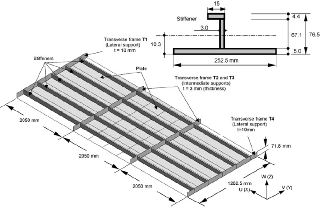
Rigo et al. (2003) considered a plate stiffened with L-shaped stiffeners, all fabricated from aluminium and joined by welding, for finite element analysis. The same model is considered in the investigations held by the authors. The model and its dimensions are illustrated in Fig. 1. One should pay attention that XYZ is the coordinate system and the U-V-W corresponding displacements.
>
Finite element code and adopted elements
All the analyses are held using ANSYS commercial finite element code. The element SHELL 181, among the element library of ANSYS is selected for meshing the stiffened plate model. SHELL181 is well suited to model linear, warped, moderately-thick shell structures. The element has six degrees of freedom at each node: translations in the nodal x, y, and z directions and rotations about the nodal x, y, and z axes.
>
Mechanical properties of material
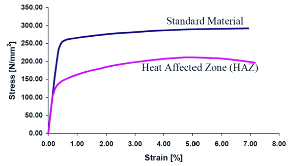
Models are made in aluminium alloy AA6082 temper T6, which its stress-strain curve is selected based on experimental results of Aalberg. The stress-strain curve of this alloy is represented in Fig. 2.
The mechanical properties of this alloy are also listed in Table 1.
[Table 1] Mechanical properties of analysis materials.
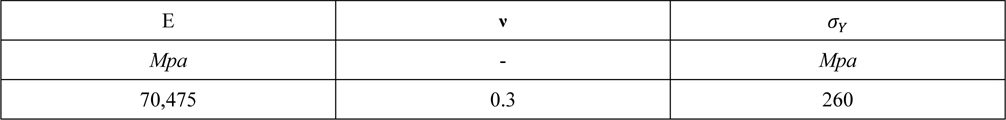
Mechanical properties of analysis materials.
Initial imperfections are one of the most important factors that affect the strength of aluminium stiffened plates. There are six primary forms of initial imperfections in aluminium stiffened plates caused by welding, namely initial distortion of plating (between stiffeners), column-type initial distortion of stiffeners, sideways initial distortion of stiffeners, residual stresses of plating, residual stresses of stiffener web and softening of the heat affected zone (Paik et al. 2008). The first three above-mentioned imperfection components are known as geometrical ones.
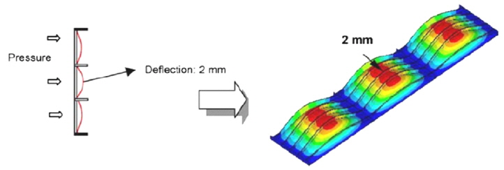
These deformations are made in panels due to building procedure. These deformations play a significant role in ultimate strength and collapse pattern of the stiffened panels as proven and investigated by Khedmati et al. (2012). They are basically modelled according to the experimental observations. For the reason of finite element modelling of the geometrical imperfections Rigo et al. (2003) have proposed a simple procedure. A uniform lateral pressure is applied first on the stiffened plate model and a linear elastic finite element analysis is carried out. From a single analysis the lateral pressure corresponding to a maximum plate deflection of 2
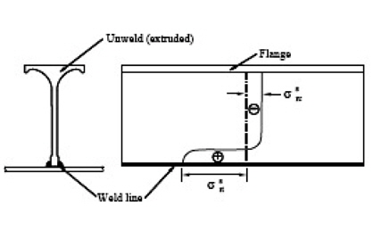
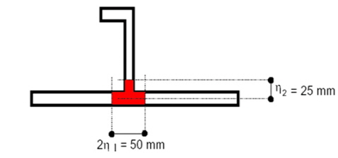
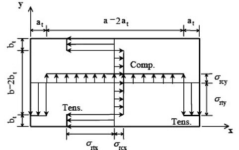
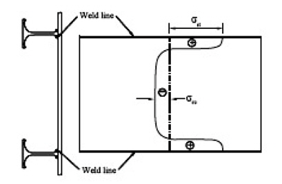
In present investigation the softening of the heat affected zone is considered for all models assembled by welding. Furthermore, the residual stress is considered in both plates and stiffeners in case of some of the models (A and A+C) and in plating only in case of some other models (B and B+C). In order to incorporate the residual stresses into the models, the instructions proposed by Paik based on empirical observations and measurements are followed. According to Paik (2008), the best welding residual stress distribution for aluminum stiffened plates can be found in Fig. 4, however, it is proposed that stresses in y direction could be ignored against the stresses in x direction.
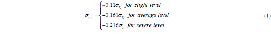
The sketch of the compressive residual stress distribution in the plating between the stiffeners is presented in Fig. 5(a) and the distribution of the same stresses in the stiffeners’ web is presented in Fig. 5(b). It should be noted that, the tensile and compressive residual stresses are in equilibrium with each other in each section. Furthermore, the (+) sign represents the tensile residual stresses and (−) the compressive residual stresses in this Fig.
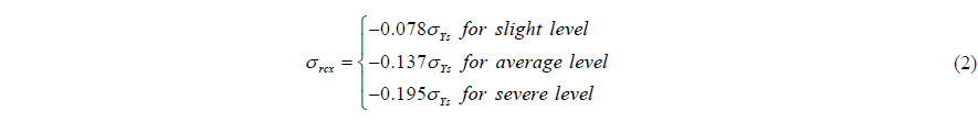
The quantitative amount of compressive residual stress in the plating between the stiffeners and stiffeners web, could be achieved by Eqs. (1) and (2) for aluminum AA6082-T6, respectively. It is worth noting, before conducting a nonlinear F.E. analysis in ANSYS the initial stress which is calculated from the equations for plate and stiffeners are applied to the model’s elements as initial condition or initial state (ANSYS user’s manual, 2007).

>
Worked-out models with respect to weld induced HAZ
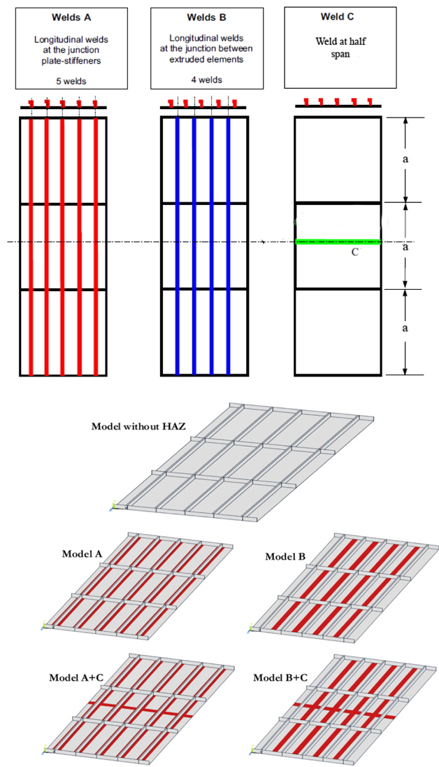
In order to distinguish the weld effects on the behaviour of the stiffened plates, five models with different HAZ arrangements, as depicted in Fig. 6, are planned.
The description of these models is given as follows: Reference model (WHAZ): the model without considering any Heat-Affected Zone (HAZ). Model A: the model with five longitudinal welds along the junction lines between the plate and five stiffeners. Model B: the model with four longitudinal welds at the intersections between the plate and five extruded elements. Model A+C: the model in which in addition to the welds as described in case of the model A, one line of transversal weld C also exists. Model B+C: the model in which in addition to the welds as described in case of the model B, one line of transversal weld C also exists.
HAZ width equals to 2 × 25
LOADING CONDITION OF COMBINED IN-PLANE UNIAXIAL COMPRESSION AND LATERAL PRESSURE
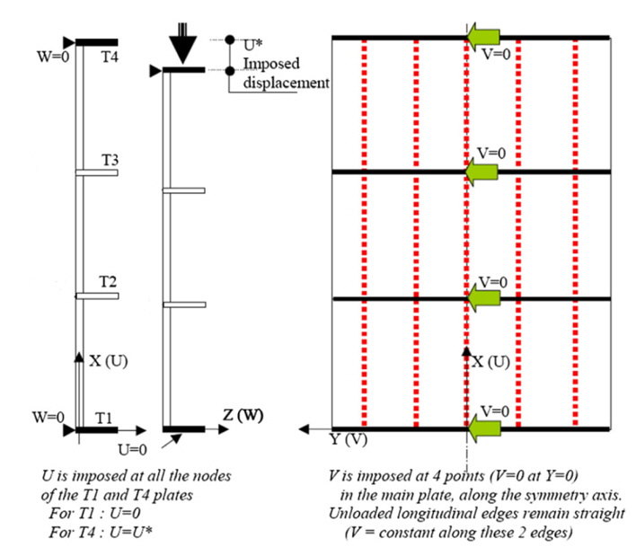
The boundary conditions in the present FE computations exactly follow those that have been implemented by Rigo et al. (2003), except that in this study the W degree of freedom on the nodes of T2 and T3 frames are not restrained, because in this study they are not intended to be rigid frames like T1 and T4. They are generally as follows:
The boundary conditions of the stiffened plates are assumed to be simply supported along the two longitudinal (unloaded) edges, which are also kept straight (constrained). The loaded edges are restrained from rotation and an axial displacement is also prescribed on them (i.e., W = V = 0 and θy = 0 on both loaded edges, with U = 0 on one loaded edge and U = U* on the other loaded edge). At these two loaded edges, the stiffener cross-section remains plane as the stiffened plate is supported by stiff transverse frames. The two end frames (T1 and T4) are assumed to be perfectly rigid (Fig. 1) and are modelled by thick transverse plates. Their dimensions are 1262.5 × 71.8mm2, while they have a thickness of 10mm. Besides, at the intermediate support locations, there are T2 and T3 frames with a thickness of 3mm (Fig. 1). These two intermediate frames together with the other two end plates provide support for the five longitudinal stiffeners. The sideways deformation of the central longitudinal stiffener would be not allowed at its crossings with the transverse frames. This means that V is restrained at 4 points in the main plate, along the symmetry axis (Fig. 8). Furthermore, unloaded longitudinal edges remain straight (V = constant along these two edges). Due to presence of stiff transverse frames, the displacements (W) along Z-axis of these two end transverse plates are not allowed. W = 0 is assumed for all the nodes at the intersection between the main plate and the two end transverse support plates (Fig. 8).
In case of pure in-plane compression, uniform in-plane displacement is imposed on one of the loaded edges while the other loaded edge is restrained against in-plane movement. When lateral pressure exists in addition to in-plane compression, first the lateral pressure is applied incrementally up to the relevant level and then uniform in-plane displacement is exerted on the model again in an incremental way.
>
Verification of the code and modeling
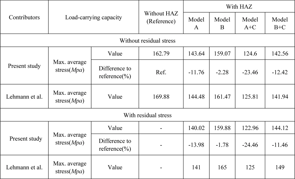
One of the most important parts of any finite-element analyses is verification of the code and modelling procedure. For this reason, the results of present modelling and analyses are compared to the results of Ultimate Strength Committee III.1 of ISSC’ 2003, on the same panel.
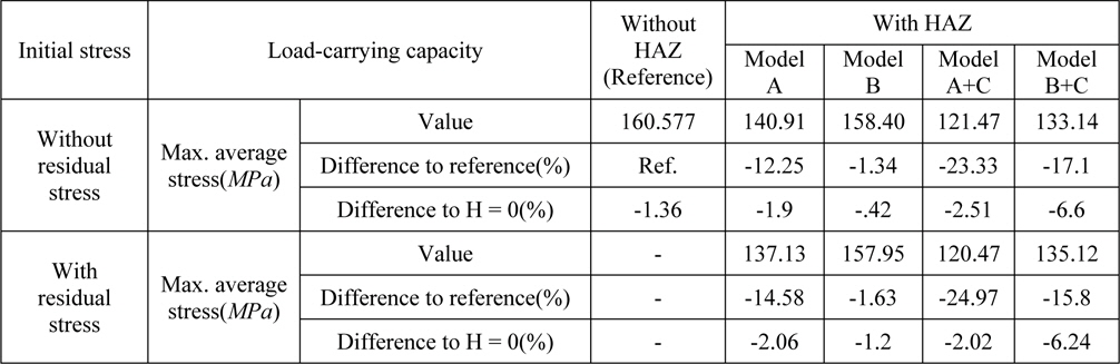
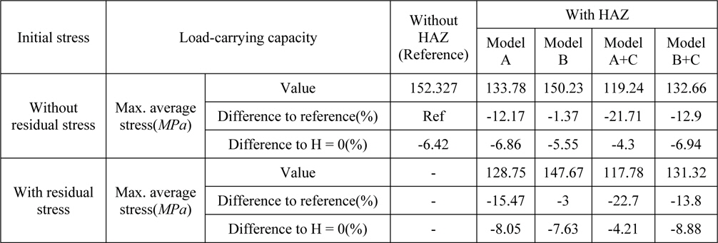
As it is presented in Table 2 good agreement is observed between the analysis results of corresponding models for the models without considering residual stresses. Likewise, the verification of the results of the analyses considering residual stresses is included in the Table 3 of this paper. It should be mentioned here that the performed analyses for verification purpose are based on the boundary conditions described in the verification or calibration section of the Committee III.1 ‘Ultimate Strength’ of ISSC’2003. This means that the nodes located on the middle transverse frames (T2 and T3 frames) are restrained from moving in
[Table 2] Comparison between the results of analyses done by researchers.
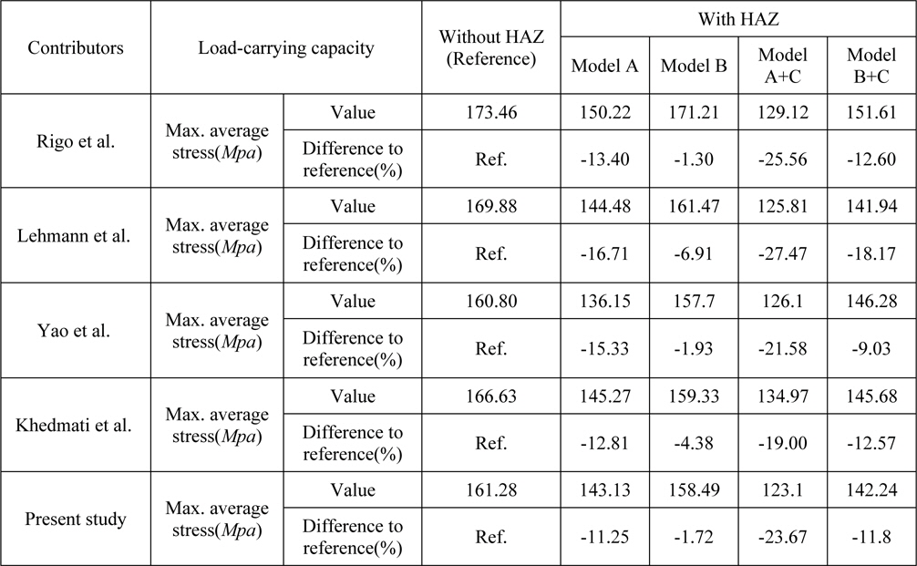
Comparison between the results of analyses done by researchers.
Ultimate strength of analyzed models subject to pure compression (lateral water height = 0).
In the analyses conducted in the present study, one aluminium panel with predefined geometrical specification has been considered and the effects of different factors have been investigated based on complicated finite-element modelling and analysis. The effects of welding on the strength of the models under different load cases have been investigated.
The results of these analyses are presented in different sets of tables and Figures, in order to facilitate the study and comparison of the results and to enable the reader to distinguish the influences of welding on the behaviour of the stiffened aluminium plate. In this regard, Tables 3, 5, 7, 9 and 11 demonstrate the results of the analysis cases under combined longitudinal compression and different levels of lateral water pressure of zero, 2.5
[Table 5.] Ultimate strength of models in analysis case with 2.5m lateral water height.

Ultimate strength of models in analysis case with 2.5m lateral water height.
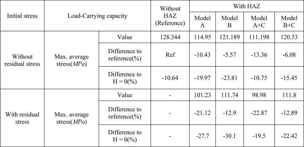
[Table 7.] Ultimate strength of models in analysis case with 5m lateral water height.

Ultimate strength of models in analysis case with 5m lateral water height.
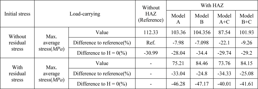
[Table 9.] Ultimate strength of models in analysis case with 10m lateral water height.

Ultimate strength of models in analysis case with 10m lateral water height.
[Table 11.] Ultimate strength of models in analysis case with 12.5m lateral water height.

Ultimate strength of models in analysis case with 12.5m lateral water height.
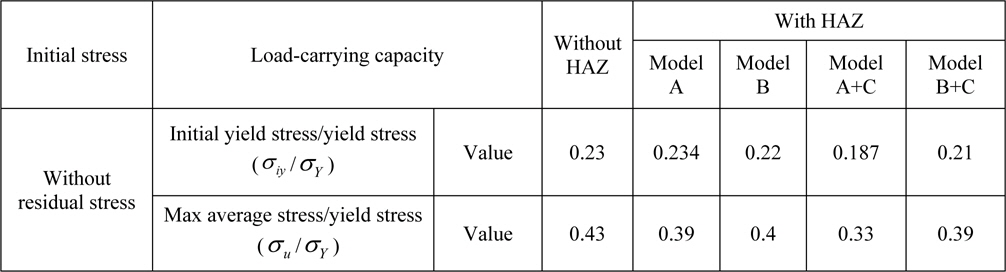
Furthermore, the Tables 4, 6, 8, 10 and 12 present the stress ratio results of analysis cases under combined longitudinal compression and different levels of lateral water head of zero, 2.5
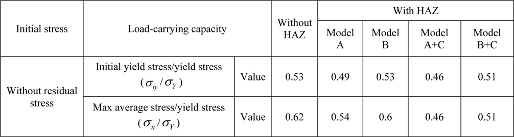
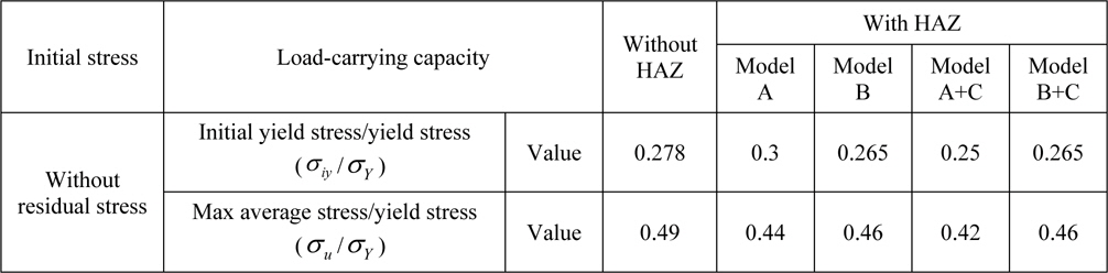
[Table 4.] Comparison between ( σiy / σY ) and ( σu / σY ) for analysis case of pure compression.
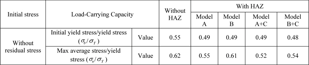
Comparison between ( σiy / σY ) and ( σu / σY ) for analysis case of pure compression.

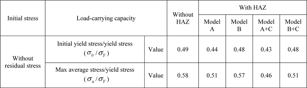
Comparison between ( σiy / σY ) and ( σu / σY ) for analysis case of 2.5m lateral water height.

Comparison between ( σiy / σY ) and ( σu / σY ) for analysis case of 5m lateral water height.

Comparison between ( σiy / σY ) and ( σu / σY ) for analysis case of 10m lateral water height.
Comparison between ( σiy / σY ) and ( σu / σY ) for analysis case of 12.5m lateral water height.
>
Load case of pure compression (Lateral water height: 0m)
According to Table 3, the reference model presents the highest ultimate strength. Among the models with HAZ, model B (consisted of extruded stiffeners) is the most efficient model. In this loading situation, adding a transverse weld line. Model A and B leads to noticeable strength reduction.
Table 4 presents the comparison between the non-dimensional yielding strength and ultimate strength of the models. In all the models containing HAZ, yielding starts at the same level of axial stress. This denotes that the initiation of yielding, in this load case, follows a similar pattern in all the models. However, with further increase in the axial loading, different arrangement of HAZ leads to different collapse and yielding patterns.
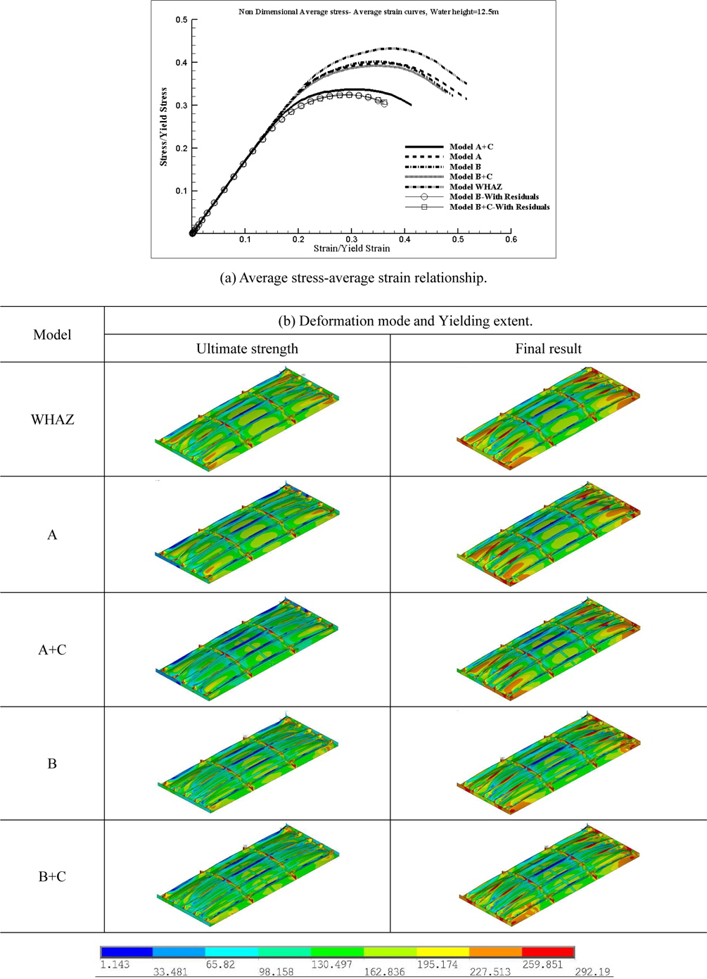
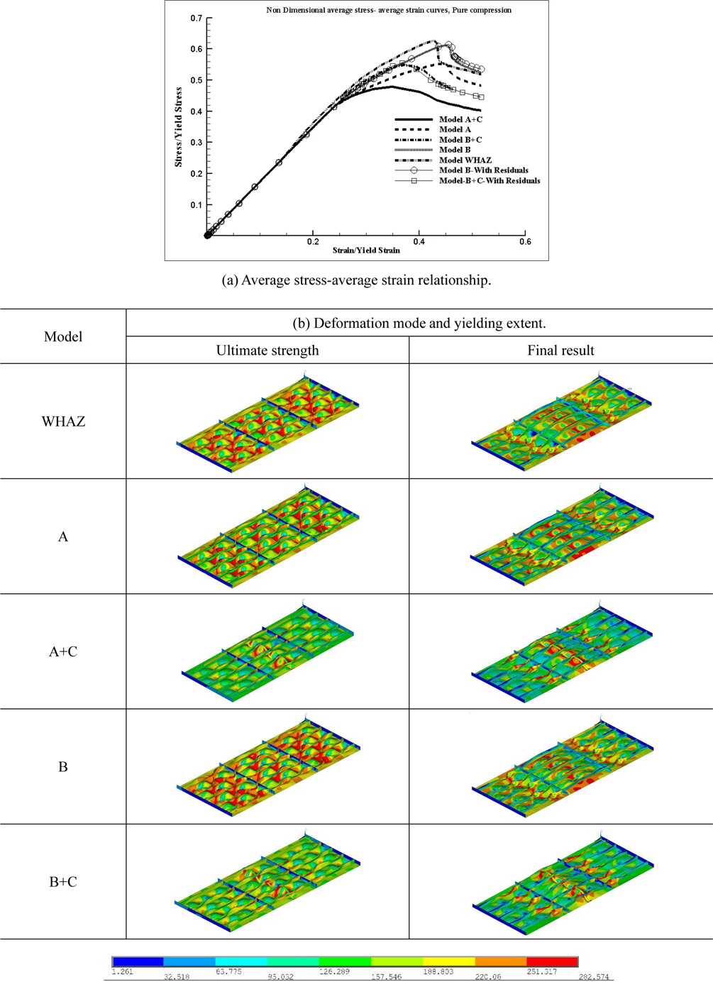
Fig. 9, provides the graphical information of the average stress-strain curve, as well as the deformation mode and yielding extent of the models at ultimate strength and final stage of analysis. It is understood from Fig. 9 that severe and vast yielding of plates and stiffeners occurs in the model A, B and WHAZ; however, model A+C and B+C experience folding mode deflection and accumulation of yielding in the vicinity of transverse weld line. This form of deflection is the main reason for significant strength reduction of models A+C and B+C.
At the final stage of analysis all the models collapse due to severe tripping occurrence in two side spans and accumulation of yielding at middle span. This accumulation of yielding at the middle span in models A+C and B+C, at presence of a weak zone at the middle span leads to folding of plating and therefore hastens the collapse of panel.
Table 3 demonstrates the effect of residual stress on the strength of models. In this loading situation, the simulation of welding residual does not result in significant change in ultimate strength of the models. Moreover, it is surprising to see consideration of residual stresses in the analysis cause raise of strength in model B and B+C. A logical justification would be made with respect of the location of tensile residual strength strip in the models. In B and B+C, it is located in the middle of plating between stiffeners; however, in the models A and A+C, it is located at the edge of plating between stiffeners. The stress-strain curve of the models B and B+C-with residuals are included in Fig. 9(a) in order to provide an overall look on the effect of residual stresses on the trend of stress-strain curve. It is understood that theses stresses do not affect this trend.
>
Load case of lateral water height = 2.5m
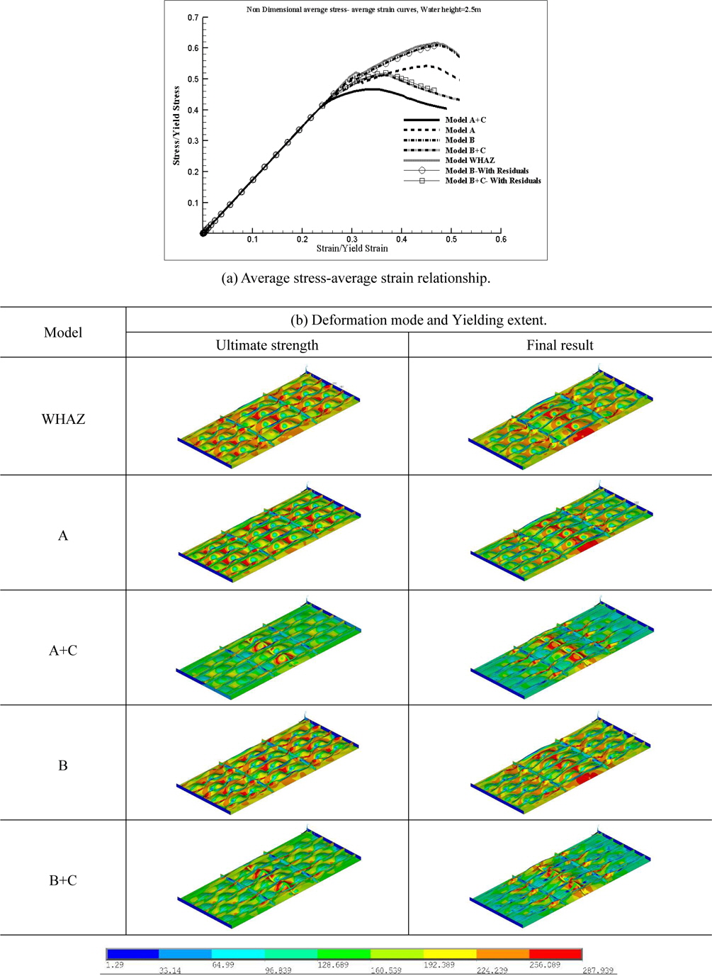
According to Table 5, when the slight lateral water height of 2.5 meter is exerted on the models, the strength of all models reduces, Compared to the case of pure in-plane compression. This comparison is included in a separate row of the Tables 5, 7, 9 and 11. A slight reduction of strength is observed in all the models at this level. The maximum strength reduction is related to model B+C in this case.
Table 6 indicates that the yielding strength varies in this lateral pressure level among the models unlike the case of pure compression. Model A+C has the lowest yielding strength. Furthermore, in model A+C and B+C the yielding begins at the ultimate strength stage. In order to find out the reason to this, the yielding extent of these models in Fig. 10(b) should be observed. According to this figure, the yielding begins very severely around the transverse weld line in association of large deformation of this weak zone. In case of other models (WHAZ, A and B), the yielding begins in the vast areas of plating and stiffeners. At the final stage of analysis, the severe yielding and tripping of stiffeners at the side spans is observed, as it is seen in the case of pure compression, except that they occur in place closer to transverse stiffeners.
As it is read from Table 5, at this slight level of lateral water pressure, the strength of all models slightly decreases. Like the case of pure compression, due to placement of tensile residual stress strip, the strength of model B and B+C is whether more than or equal to their corresponding without residual stress models. The strength reduction compared to case of pure compression also shows slight dependence on residual stresses. Fig. 10(a) facilitates the comparison of the results in this case.
>
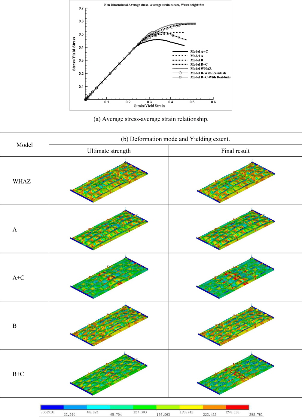
Load case of lateral water height = 5m
In this load case except for model B, in other welded models a significant divergence of the ultimate strength is observed when the results are compared to reference model, with highest divergence related to model A+C. Furthermore, due to existence of 5
According to Table 7, model WHAZ, A and B show after yielding load carrying capacity, while, like the case of 2.5
Fig. 11(b), denotes that in model A, B and WHAZ the ultimate strength and final stage of analysis are very close to each other from the stress distribution viewpoint. These models are mainly collapsed by yielding and tripping of stiffeners near the transverse frames, especially near the loaded ends. No accumulation of plasticity is noticeable in plating of three models; however, in model A+C and B+C the folding deformation of mid-span and plasticity accumulation in the vicinity of transverse weld line are significant.
According to Table 7, with consideration of residual stresses, the ultimate strength of all the models, with no exception, reduces. However, like the former cases, they are not very much effective in the strength of models compared to the HAZ arrangements and geometrical imperfections. See Fig. 11(a) for their effect on the average stress-strain curve too.
>
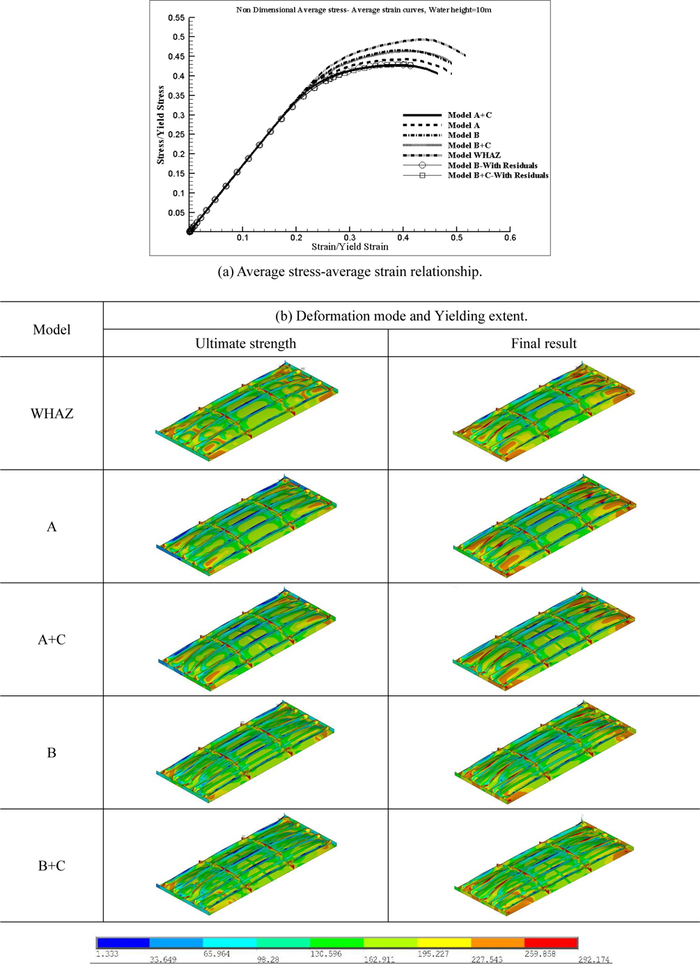
Load case of lateral water height = 10m
Table 9 shows that the reduction of strength compared to the case of pure compression, is remarkable in this case. The maximum percentage of the reduction is observed in model B, which has the maximum highest strength among the welded models. Therefore, it could be inferred that the collapse pattern of the panels is fully under distinguished by different levels of lateral water height. In this case, model B is the most efficient model among the welded models and the model A+C is still the weakest model and represents the maximum strength reduction.
According to Table 10, the yielding strength of the models are severely reduced and unlike the two previous cases with lateral pressure, none of the models has the same yielding and ultimate strength. This lateral pressure results in faster occurrence of yielding; while the after yielding load carrying capacity is remarkable in this case.
Fig. 12(b) shows that in this case, the collapse pattern of all the models are the same. It means that models experience membrane type deflection, which is followed by tripping and yielding of stiffeners at their junction with end transverse frames until they reach to ultimate strength stage. In this stage intensive yielding at the intersection of the transverse frames and longitudinal stiffeners is observed. At the final stage of analysis the areas of yielding in the frames and stiffeners become vaster. Unlike the former cases, the folding type deflection and accumulation of plasticity is not seen near transverse weld line.
The information in the Table 9 convey the fact that in this lateral pressure level the effect of residual stresses on the ultimate strength is noticeable especially in case of model A and A+C. For example, in case of model A, due to this type of HAZ arrangement, model loses almost 10 percent of its strength and due to the residuals it loses another 11 percent of its strength. Therefore, in this load case the HAZ arrangement and residual stresses are of the same importance in reduction of strength. Fig. 12 (a) provides a better insight over the effect of residual stresses. It is noticeable to see that they do not change the trend of stressstrain curve, because it is determined by the lateral water height. By the way, this figure indicates that the transverse weld line is not important in this case. This is because the strength of panels is less than the yield strength of HAZ material and the panels deflect like a membrane.
>
Load case of lateral water height = 12.5m
Table 11 represents the data of ultimate strength of models in this case, both with and without residual stresses. The same information expressed on the previous section (Load case of lateral water height = 10
This effect is more in model A and A+C compared to B and B+C, due to presence of residual stresses in the stiffeners. Furthermore, in the Fig. 13(a) the stress-strain curve illustrates this point. Table 12 provides data on the yielding strength and post yielding load carrying capacity of models, which are both significant, the former due to its small amount and the later due to its high amount. This means that the large deflections and distortions of the models hastens yielding, until the collapse of panel and spread of yielding in the transverse frames and longitudinal stiffeners at ultimate strength stage (as it is illustrated in the Fig. 13(b)), there remains some load carrying capacity. The yielding pattern is the same as what was explained in the previous section; except that the yielded areas are vaster and more intensified.
In this paper, the results of the sophisticated numerical studies held to investigate the effect of weld on the strength of the aluminum stiffened plates are preselected. The selected finite element models are subject to combined in-plane compression and lateral pressure.
The main conclusions in brief are: The increase of lateral water pressure leads to decrease of ultimate strength of the models. The arrangement of the weld lines does not affect this overall trend. Both the type of the stiffeners (extruded or welded up) and welding arrangements influence the post buckling behavior and ultimate strength of the models. In case of pure compression, the existence of a transverse weld line will cause the collapse pattern to change to a mode in which tripping of the stiffeners and a further spread of yielding in stiffeners as well as local accumulation of the yielding in vicinity of the transverse weld line is experienced. The magnitude of the lateral pressure, existence and arrangement of the weld lines, are the main factors affecting the postbuckling behavior and ultimate strength of the models. Folding deflection in the central span is frequently observed in the models with transverse weld line. Under different level of lateral water pressure this form of deflection accompanied by the plasticity accumulation results in significant strength reduction of models with transverse weld lines compared to the other models. Tripping and yielding of stiffeners are the major collapse modes observed in all models in ultimate strength and final stage of analysis. For any value of the lateral water pressure, the model A+C displays the least ultimate strength. With all the levels of lateral water pressure, model WHAZ or B displays the maximum ultimate strength. The overall trend of average stress-strain curve is mainly under the influence of the amount of lateral water height. Regarding the effect of residual stress some points are inferred: 1. Taking the residual stresses into account does not affect the overall trend of the Average stress-Average strain curve under different level of lateral pressure. 2. At pure compression load case, the reduction of strength is observed in model A and A+C, an increase of strength is observed for model B and B+C. It seems as if a tensile stress strip in the middle of the plate field improves the strength behavior of the panel. However, in A models, the tensile stress strip is at the boundary of plates thus resulting in decline of strength. 3. At low lateral water height, the simulation of residual stresses leads to minor strength reduction in models A and A+C, and minor strength increase in the B and B+C. 4. As the lateral pressure increases the divergence between the result of the model with and without residual stresses increases. This denotes the importance of residual stresses at high lateral pressure load cases; while it is of minor importance at low lateral pressure and pure compression load cases. 5. At the highest lateral water height considered for this study (12.5m), models with residual stress lose almost half of their strength compared to case of pure compression. Therefore, for the panels, which are intended to operate in deep seas some other welding methods except fusion welding is appreciated. 6. Generally, the contribution of the residual stresses to change in strength is more remarkable in model A and A+C compared to B and B+C. 7. The residual stresses do not affect the overall yielding, deformation, collapse and stress-strain curve of the models.