


Swarm intelligence, as an emerging intelligent computing technology, has been the focus of attention of artificial intelligence researchers. In 2002, Passino [1] who was inspired by the social foraging behavior of
In recent years, the BFO algorithm has gradually aroused the wide attention of experts and scholars at home and abroad, and corresponding research about the theory and its application has been launched. Abraham et al. [2], a research team on the BFO algorithm carried out a series of studies, and concluded that a reproduction operator in the BFO algorithm is conducive to improve the convergence speed of the algorithm. They used genetic algorithms and a differential evolution algorithm to improve the ability of searching for the global optimum of the BFO algorithm [3]. The improved algorithm has been successfully applied to the optimization of the PID parameter. Also, Das et al. [4], Indian scholars, analyzed the influence of adaptive step size on its convergence and stability, from a theoretical point of view. However, their analysis was based on certain assumptions, which only consider the chemotaxis operation of a single particle in one-dimensional continuous space. A fast bacterial swarming algorithm based on the improved quorum sensing mechanism was proposed by Ying et al. [5], and applied to image compression. In addition, Li and Yang [6] proposed a bacterial colony optimization algorithm based on the improved mechanism of BFOA, and proved that the algorithm is effective. Tripathy et al. [7] solved the problem of optimal power flow by the BFOA. The BFO and other intelligent algorithms [8-10] are also combined, in order to improve the algorithm applied to predictive control [11], image clustering [12], and multi-objective optimization [13].
Ⅱ. THE CLASSICAL BFO ALGORITHM
The foraging strategy of
Chemotaxis is achieved by swimming and tumbling. When a bacterium meets a favorable environment (rich in nutrients, and noxious free), it will continue swimming in the same direction. When it meets an unfavorable environment, it will tumble, i.e., change direction. Let S be the total number of bacteria in the population, and a bacterium position represents a candidate solution of the problem and information of the i-th bacterium with a
where
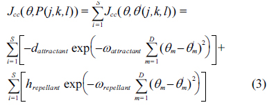
The health status (fitness) of each bacterium is calculated after each completed chemotaxis process. The sum of the cost function is
where
>
C. The Elimination and Dispersal Operation
C. The Elimination and Dispersal Operation The chemotaxis provides a basis for local search, and the reproduction process speeds up the convergence, which has been simulated by the classical BFO. While to a large extent, chemotaxis and reproduction alone are not enough for global optima searching, since bacteria may get stuck around the initial positions or local optima, it is possible for the diversity of BFO to change either gradually or suddenly to eliminate the accident of being trapped into the local optima. In BFO, the dispersion event happens after a certain number of reproduction processes. Then, some bacteria are chosen to be killed according to a preset probability Ped or moved to another position within the environment.
where
>
A. Analysis of the Elimination and Dispersal Step in BFOA
The elimination and dispersal operator is an indispensable link in BFOA. With the probability Ped, each bacterium eliminates and disperses in order to keep the number of bacteria in the population constant. If a bacterium is eliminated, another bacterium is simply dispersed to a random location on the optimization domain. As per the optimization of multi-modal function, the bacterium is easily trapped into local optima and it is difficult to escape. Thus, the convergence speed and accuracy of the algorithm is affected. The elimination-dispersal operator helps bacteria that are trapped into local optima to escape. A greater probability of migration can provide more opportunity for the bacteria to escape from the local optimum. However, at the same time, the solution of the local optimum brings a new problem, called “escape”. It results in reducing the convergence speed and accuracy of the algorithm. Such a situation is not expected to exist.
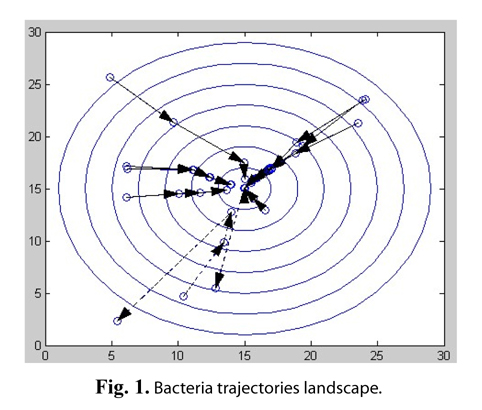
For example, the classical BFO algorithm is applied into solving a simple nonlinear function: z = (x − 15)2 + (y −15)2, where x∈[0,30], y∈[0,30]. Assuming that the total number of bacteria is 10 in the population, the number of evolution generations is 4, the chemotaxis operation is performed 10 times in each generation, and the probability of elimination and dispersal is 20%, the bacterial individual trajectories are shown in Fig. 1.
This function has an optimal solution that z equals 0, where x = 15, y = 15. The origin shows the position of the bacterial individual in Fig. 1, and the arrow lines show the change in position of individual bacteria, after a generation optimization. As shown in the figure, most bacteria are constantly moving to the optimal position. However, some bacteria marked as dashed lines at or close to the optimal value have suddenly moved away from the optimum value, due to the operation of elimination-dispersal.
How to avoid escaping? In the optimization process of an individual bacterium, if the individual bacterium that is selected for the elimination-dispersal operator is found at, or close to, the global optimal solutions, escape will essentially happen. Thus, in order to avoid the escape, we should prevent such bacteria from being selected.
Therefore, the elimination-dispersal operator needs to be improved. The bacterial individuals are sorted in accordance with their current fitness values. The elimination-dispersal operator selects bacterial individuals, according to the probability of Ped, only from the fitness value ranked behind some bacteria individuals; while the others will not be selected, because the bacterial individual standing in the front of the individual is found at, or very close to, the global optimal solution. Thus, escape can be effectively avoided. By increasing generations, bacterial individuals continue to move closer to the optimal position. The proportion of the elimination and dispersal steps of bacteria should be appropriately reduced. Let Q be the percentage of elimination and dispersal of bacteria, and its initial value is 1. The generation is the chemotactic generation counter, and its initial value is 0. An elimination and dispersal step is done after every ten generations in the algorithm, and the scope of the elimination and dispersal should be reduced in every 20 generations. This means that if generation MOD 10 = 0, then the elimination and dispersal step can be done. Let ged = generation DIV 20, Q = 1 − (2ged*L), where L is the percentage of initial value of bacteria that do not participate in the elimination and dispersal. As the generations increase, ged increases, and the percentage of elimination and dispersal decreases. Therefore, the occurrence of escape can be avoided, and the speed of convergence can be greatly improved.
>
B. Analysis of the Chemotaxis Step in BFOA
The chemotaxis operation is one of the most important steps in BFOA. During the chemotaxis operation, bacteria are continually swimming to find the optimal solution to the problem. At the initial location, a bacterium tumbles to take a random direction and then measures the food concentration. After that, it swims a fixed distance and then measures the concentration there. This action of tumble and swim constitutes one chemotactic step. If the concentration is superior at the next location, the bacteria will take another step toward that direction. If the concentration at the next location is lesser than that of the previous location, the bacteria will tumble to find another direction, and swim in this new direction. This process is carried out repeatedly, until the maximal number of steps, which is limited by the lifetime of the bacteria.
In the chemotactic steps, step size is an important parameter, when the bacteria select to swim forward in a certain direction [14-17]. How to set the step size? In the conventional BFOA, a simply fixed step size was selected based on experience. However, such treatment often makes the convergence speed of the algorithm slow, or falls into a local optimum. Thus, there should be better parameter values.
The selection of the step sizes is a critical issue, throughout the design process of the algorithm. If the step sizes are too small, the search will be trapped into local optima. On the other hand, if the steps are too long, the search will miss the global optimum. After taking this into consideration, equations for long tumble size (LT), short tumble size (ST), and swim size (SW) were defined. Almost every user intervention is needed, due to it being automatically updated during the process.
The BFOA was applied, to solve the Schaffer function.
This function has a global optimum, where
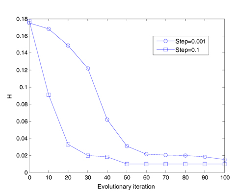
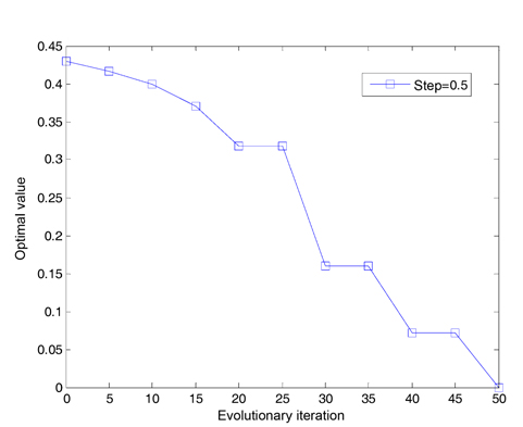
We assume that the total number of bacteria is 50 in the population, the dimension of the solution space is set to be 2, the maximum number of steps in the same direction is 4, the depth of the attractant and the height of the repellant are both 0.1, the width of the attractant is 0.2, the width of the repellant is 10, the initial probability of the elimination-dispersal is 30%, the evolution generation is 100, the step size is 0.1 and 0.001, respectively, and the mean minimum value H of function is plotted as shown in Fig. 2, after the algorithm is implemented 20 times. In addition, assume that the evolution generation is 50, and the step size is 0.5. The mean minimum value H of the function is plotted in Fig. 3, after the algorithm is implemented in one run of every 10 generations.
In Fig. 2, we can get a result that if the step size is set to be 0.1, the convergence speed of the algorithm is very high, but no longer converges after 60 generations. If the step size is set to be 0.001, the convergence speed of the algorithm is apparently reduced after 100 iterations. It has not yet met the expected precision. In order to reach the required accuracy, the iteration times must be increased, and its efficiency will be greatly reduced.
After 20 generations have evolved in Fig. 3, the curve decreases stepwise every 10 generations, and the optimal value converges once. The reason is that the algorithm is designed to reduce half of the step sizes every 10 generations. Obviously, the small step length can improve the accuracy of the algorithm.
From the above discussion, it is clear that the selection of the step sizes is a critical issue, throughout the design process of the algorithm. If the step sizes are too small, the search can be trapped into local optima. If step sizes are too long, the search will miss the global optimum. Bacteria with larger step sizes will move in the entire search space, while the bacteria with smaller step sizes can do fine only in search around local optimal solutions. Hence, the chemotactic operator (i.e., the step size) should be chosen, in order to allow the bacteria to explore the entire search space, and search effectively around the potential solutions. Therefore, the fixed step size cannot meet the requirements of accuracy and convergence speed at the same time.
It is convincing that variable step sizes can not only meet the high convergence speed, but also satisfy the requirement of high precision. By means of the variable step size, we let the initial value of the step size, STEP = 0.002R, where R is the optimal interval width. It is gradually reduced, along with an increasing number of iterations. In an early iterative algorithm, the step size decreases slowly, but it shrinks faster and faster, along with an increasing number of iterations. Thus, in the early algorithm execution, bacteria rush to the optimal solution space, and accelerate the convergence speed. This improves the convergence precision, with the step size decreasing rapidly.
We briefly outline the novel BFO algorithm step-bystep, as follows.
[Step 1] Initialize parameters S, try_number, STEP, dattractant, ωattractant, hrepellant, ωrepellant, Ped, L.
where,
S: the number of bacteria in the population, try_number: the maximum number of steps in the same direction,STEP: the step size,dattractant: the depth of the attractant,ωattractant: the width of the attractant,hrepellant: the height of the repellant,ωrepellant: the width of the repellant,Ped: elimination-dispersal with probability,L: the percentage of the initial elimination-dispersal.
[Step 2] Compute the initial fitness values of each bacterium.
[Step 3] Let i = 0, generation = 0, t = 0, Q = 1.
[Step 4] Chemotactic operator and quorum sensing mechanism: [SubStep 4.1] If generation MOD 10 == 0, {g= generation DIV 10, STEP=STEP/2g}, [SubStep 4.2] let Jlast be represented as the current fitness value, [SubStep 4.3] get the new fitness value Jnext, when a bacterium runs length unit STEP in the random direction, [SubStep 4.4] Jcc, the influence value of other bacteria on an bacterium, is calculated according to Step 2, let Jnext = Jnext + Jcc, [SubStep 4.5] if t < try_number, then t = t +1, else t = 0, go to SubStep 4.8, [SubStep 4.6] if Jnext is superior to Jlast, then Jlast = Jnext, else t = 0, go to SubStep 4.8, [SubStep 4.7] to walk step length STEP in the same direction, Jnext = fitness value of the new position, go to SubStep 4.4, [SubStep 4.8] let i = i + 1, if i < S, then go to SubStep 4.1, else i = 0, generation= generation + 1, go to Step 5.
[Step 5] Reproduction steps: [SubStep 5.1] Reproduction operator will be done every 5 generations, [SubStep 5.2] sort descending order by the current fitness values of each bacterium, [SubStep 5.3] locations of one half of bacteria, with inferior fitness values, are replaced by the other half, with superior fitness values.
[Step 6] Elimination and dispersal operator: [SubStep 6.1] Elimination-dispersal operator will be done every 20 generations, [SubStep 6.2] update range of the current elimination and dispersal Q = 1 – (2ged*L), if Q < 0, then let Q = 0, [SubStep 6.3] sort descending order by the current fitness values of each bacterium, [SubStep 6.4] let Sed = S*Q, select bacterial from queue rear sorted Sed, in accordance with the probability of the elimination and dispersal Ped, to take the elimination- dispersal operator
[Step 7] Check the terminal condition (usually reaches a predetermined evolution generations or good enough fitness values), and if the terminal condition is satisfied, output optimal solution and algorithm terminates; otherwise, go to Step 4.
To illustrate the performance of the improved BFO algorithm, we present the results of the improved BFOA, using a test-suite of five well-known benchmark functions:
1) Rosenbrock function
The local minimum of the Rosenbrock function which is two-dimensional, odd behaving, and hard to minimize, is calculated, where x∈[-2.048, 2.048]. The function has the global optimum, which is 0, when xi = 1 (
2) Rotated hyper-ellipsoid function
The rotated hyper-ellipsoid function that is unimodal is calculated, and its global minimum is
3) Ackley function
This function that is multimodal is calculated. Its global minimum is at
4) Rastrigin function
This function that is a multimodal is calculated. Its global minimum is at
5) Griewank function
This function that is multimodal is calculated. Its global minimum is at
Using a computer PC (Pentium 4/3.0 G, Memory 4 G) with OS platform for Windows 7, C programming language, the performance of the algorithm is evaluated according to the following methods: 1) with fixed evolutionary iteration, the convergence speed and precision of the algorithm is evaluated; 2) with fixed target value of convergence precision, the number of iterations of the algorithm that reaches the required accuracy is evaluated; other algorithms. and 3) the performance of the algorithm is compared to
>
A. Convergence Speed and Accuracy of the Algorithm under the Fixed Evolutionary Iterations
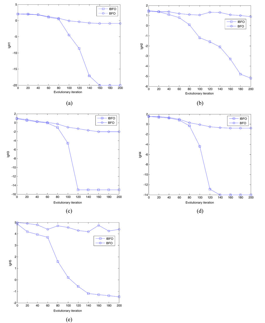
Suppose that the rest of the parameter settings that were kept in the algorithms are as follows. The total number of bacterial population is 50. The dimension of solution space for the four testing functions is set to be 2. The maximum number of steps in the same direction is 4. The number of fixed evolutionary iterations is 200. The depth of the attractant and the height of the repellant are both 0.1. The width of the attractant is 0.2 and the width of the repellant is 10. Let the initial probability of the elimination- dispersal Ped be 15%, and the step sizes STEP = 0.001R, based on the BFO algorithm. In addition, let the initial probability of the elimination-dispersal Ped be 30%, the step sizes STEP=0.002R, and L=3% in the improved IBFO. Fig. 4 presents the convergence characteristics using the basic bacterial foraging algorithm and the improved algorithm (IBFO) to run 20 times in terms of the best fitness value of the median run of each algorithm for each test function.
The figures above depict optimal results, for different test functions. We can see that the classical BFO algorithm with a fixed step size almost stops converging, when it optimizes to a certain value, or even jumps, due to the escape of bacteria; whereas, the improved BFO (IBFO) algorithm overcomes these shortcomings. With an increasing number of iterations, and decreasing step sizes, the accuracy of the algorithm is greatly improved, and the convergence speed of the algorithm is significantly increased. Therefore, the improved algorithm performance is much better than that of the basic algorithm.
>
B. Evolutionary Iterations under the Fixed Convergence Accuracy of the Algorithm
Experimental parameters of the evolution iterations in the fixed convergence precision are set as follows: the target convergence precision is 0.0001; the maximum number of iterations is 600; and the other parameters are as shown above.
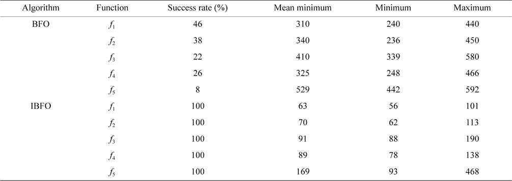
It is shown in Table 1 that five test functions independently operate 60 times, to acquire the number of iterations under the specified convergence accuracy, where the success rate is the number of runs to the target accuracy divided by the total number of experiments.

The number of iterations under the specified convergence accuracy for benchmark functions f1, f2, f3, f4, and f5
As shown in Table 1, the success rate of the basic BFO algorithm is small. The maximal success rate is only 46% in the four test functions, whereas the success rate in the improved algorithm (IBFO) is 100%. The improved algorithm (IBFO) in the case of successful convergence is better than the basic algorithm, in the required minimum number of iterations, and the maximum number of iterations. The above results indicate that the improved BFO (IBFO) algorithm is superior to the basic BFO algorithm.
>
C. Comparison with Other Algorithms
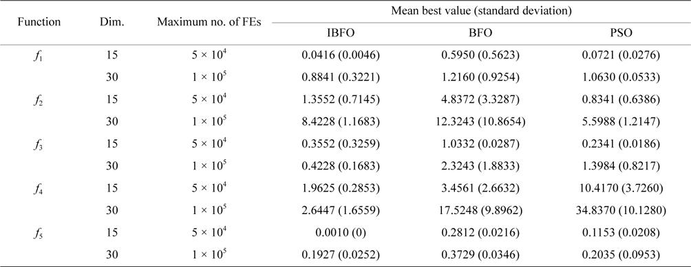
We have compared IBFO with BFO and particle swarm optimization (PSO). The comparison ends up with the condition that the number of iterations achieves 105, or the optimal value reaches the target value, i.e., 0.001. The solutions of 100 times operations of IBFO, BFO, and PSO on

Average and standard deviation (in parenthesis) of the best-of-run for 50 independent runs tested on five benchmark functions
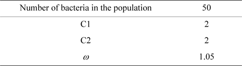
[Table 3.] Particle swarm optimization algorithm relevant parameter

Particle swarm optimization algorithm relevant parameter
The algorithm is improved in the elimination-dispersal and chemotaxis operations, based on the basic BFO. By limiting the range of the elimination-dispersal of bacteria, the escape phenomenon can be avoided and the convergence speed of the algorithm is effectively improved. Furthermore, the influence of the step size in the chemotaxis operations on the algorithm has been analyzed; the convergence speed and the precision of the algorithm with variable step size have been improved. Experiments show that the IBFO greatly improves its convergence speed and precision, and it is suitable for both unimodal and multimodal functions.