Ghost Imaging with Different Speckle Sizes of Thermal Light

Jue
Wang; Renlong
Yu; Yu
Xin; Yanming
Shao; Yanru
Chen; Qi
Zhao

doi:10.3807/JOSK.2016.20.1.008

OA학술지
Journal of the optical society of Korea

Ghost Imaging with Different Speckle Sizes of Thermal Light

DOI : 10.3807/JOSK.2016.20.1.008
Author: Jue Wang, Renlong Yu, Yu Xin, Yanming Shao, Yanru Chen, Qi Zhao
Publish: Journal of the optical society of Korea Volume 20, Issue1, p8~12, 25 Feb 2016

ABSTRACT

Ghost Imaging with Different Speckle Sizes of Thermal Light

KEYWORD

Ghost imaging , Coherence , Speckle size , Edge blur

본문

Collapse all

I. INTRODUCTION

In the past decade, ghost imaging (GI) has attracted a lot of attention. In ghost imaging, the object image is retrieved by using two spatially correlated beams: the reference beam and the object beam. The reference beam never interacts with the object and is measured with a pixelated detector. The object beam interrogates the object and then illuminates a bucket detector, with no spatial resolution. By correlating the reference beam with the bucket signal, the ‘ghost’ image is retrieved. In 1995, the first GI was found in quantum optics [1], and it was once considered as a unique phenomenon of quantum optics. However, in 2002, Bennink achieved ghost imaging with scanning of a pair of collimated laser beams [2], which sparked a debate [3-5] of whether GI was a quantum effect or not. Then a variety of thermal light sources [3-8] were used to realize GI. Recently some teams focused on the application of GI, such as GI by measuring reflected photons [9], compressive GI [10-12], GI through turbulent atmosphere [13], GI in turbid media [14]. However, only a few teams [7, 15, 16] focused on the impact of the speckle size on GI. In this paper, we theoretically and experimentally analyze the pros and cons of GI with different speckle sizes, and try to present a setup which can at the same time make the best use of the advantages and bypass the disadvantages caused by different sizes of speckles.

II. METHODS & RESULTS

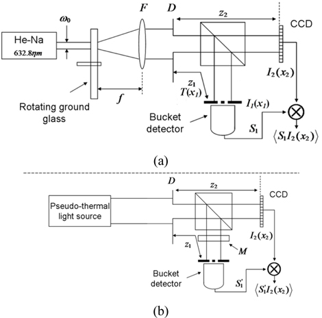
In order to get speckles with different sizes, we used the setup in [17] (see Fig. 1(a)). The laser and rotating ground glass constituted a pseudo-thermal light source. The ground glass was in the focal plane of the Lens F while D was an aperture. With the formula δx₀ = πλf / ω₀, we can get desired speckle size δx₀ by changing f of Lens. Here, λ is the wavelength of light and ω₀ represents the waist radius. The role of beam splitter is to form two spatially correlated beams. Beam 1 (the object beam) is collected with a bucket detector after illuminating the object. Beam 2 (the reference beam) never interacts with the object and measured with a pixelated detector. The distance between Aperture D and the two detectors are z₁ and z₂ respectively. Let us indicate with I₁(x₁) and I₂(x₂), the intensity distributions of the speckle fields on the object and reference planes, respectively. If T(x) indicates the transmission function, the bucket signal S₁ is

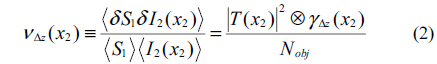
[FIG. 1.] Experimental setups for ghost imaging. (a) the traditional setup for ghost imaging. (b) the improved setup for ghost imaging.

According to the result of [7], we have the following formula

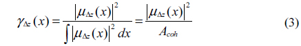
Where <⋯> indicates the average over independent speckle configurations. µ_Δz(x₁, x₂) is the cross-correlation coefficient of the electric fields at the planes z₁ and z₂. A_coh is the area of the speckle, which is related to the speckle size by . ⊗ denotes convolution, N_obj = A_obj / A_coh denotes the number of the speckles falling into the object. Eq. (2) shows that the visibility of GI [i.e., the maximum value of v_Δz(x₂)] is equal to 1/N_obj and, except for convolution effects (occurring when γ_Δz(x₂, x₁) and T(x₂, x₁) have similar widths), is independent of Δz. Another indicator to evaluate the GI is SNR [15, 16]

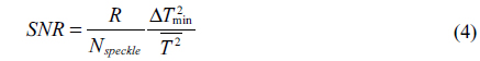
While N_speckle = A_beam / A_coh is the number of the speckles in the beam, ΔT_min is the minimum variation of the object transmission function to be detected. is the average quadratic transmission function of the object. R represents the independent sampling number. With Eqs. (2) and (4), we know that for the case of using the same average number, a larger speckle size will lead to higher visibility and SNR. However, in experiments we found that a larger speckle size will get a more blurred edge of the object as well. We call this phenomenon edge blur of GI. We will theoretically analyze the reason of this phenomenon and experimentally show the edge blur of GI in the following.

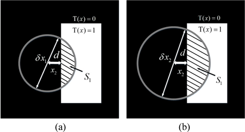
Considering the case shown in Fig. 2, there is a point x₂ where the transmission function is T(x₂) = 0, and the distance from the edge is d. δx₁ and δx₂ are the sizes of two different speckles where δx₁ < δx₂. The shaded areas indicate that the region can be received by the bucket detector. When δx₀ = D, the mutual coherence function [18] is

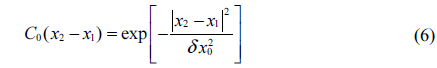
[FIG. 2.] The schematic view of the point x2 where the transmission function is T(x2) = 0.

Where I₀ is a real function representing the mean transverse intensity distribution at the source plane, varying on the large scale D the source diameter. C₀ is a real function with the property C₀(0) = 1, which dies out over the small scale δx₀ (the speckle transverse size). In the deep-Fresnel zone，the coherence factor characterizing the granular structure of the source has a Gaussian profile of the form

Here, we only consider the case z₁ = z₂. Then, we obtain the complex coherence factor and its squared modulus reads as:

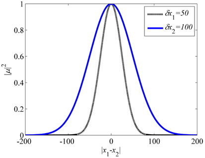
Eq. (7) illustrates that in the case where z₁ = z₂, │μ│² is a Gaussian function described by the size δx₀. The graph of │μ│² and │x₁ – x₂│ is shown in Fig. 3. We can see that for the same │x₁ – x₂│, a larger speckle leads to a bigger │μ│².

[FIG. 3.] The graph of │μ│2 vs │x1 ？ x2│.

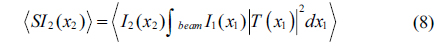
The correlation between S₁ and I₂ (x₂) is

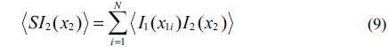
Assuming that the bucket detector is pixelated, so we obtain discrete result

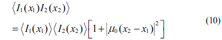
Where N denotes the number of the pixels in the shaded areas in Fig. 2. From Fig. 3 we can see that

Combining Eqs. (10) and (11), we have the result

On the other hand, from Fig. 2, the number of pixels has the relation that N_δx₁ < N_δx₂, so we obtain the final result

Eq. (13) shows two key features of GI with a pseudothermal light source: Firstly, because of the Gaussian distribution of the correlation radius of the speckle, I₂(x₂) and bucket signal S₁ are still related and the retrieved T(x₂) > 0, although the ideal T(x₂) = 0. Theoretically, when d > δx₀ / 2, the transmission function T(x₂) = 0, and we call this distance δx₀ / 2 as the width of edge blur. Secondly, while Eqs. (2) and (4) illustrate that the ghost imaging will have a higher visibility and SNR with lager speckle, Eq. (13) shows that it will bring a more serious edge blur as well.

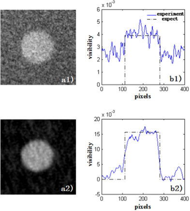
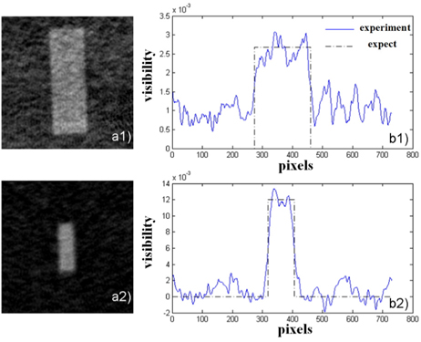
In order to experimentally demonstrate the edge blur, we implement the experiment shown in Fig. 1(a). The source is a He-Na laser (λ = 632.8 nm, ω₀ = 2 mm). By selecting different lenses (f = 50 mm and f = 100 mm, respectively), we obtain two kinds of speckle with δx₁ = 49.7 µm and δx₂ = 99.4 µm. The object was an aperture whose diameter is 900 µm. The experimental result is shown in Fig. 4. Where Panel a1 shows the 2D-ghost image retrieved by averaging R=12800 independent realizations of the speckle field (δx₁ ≈ 50 µm). Panel b1 shows the horizontal profile of the aperture (blue continuous line), this profile compares with the expected one (dotted line) and its visibility is 0.0039. Panel a2 shows the 2D-ghost image retrieved by averaging R = 12800 independent realizations of the speckle field (δx₂ ≈ 100 µm). Panel b2 shows the horizontal profile of the aperture (blue continuous line), this profile compares with the expected one (dotted line) and its visibility is 0.0156.

[FIG. 4.] The ghost imaging reconstruction of an aperture whose diameter is 900 μm. (a1) and (b1) are the reconstruction images which obtain 12800 realizations, when the speckle size of the thermal source is 50 μm. (a2) and (b2) are the reconstruction image which obtain 12800 realizations, when the speckle size of the thermal source is 100 μm.

Comparing the results with different speckles, we have the following conclusions: Firstly, compared with Fig. 4(a1), the retrieved image with larger speckle (see Fig. 4(a2)) has a higher SNR. Secondly, compared with Fig. 4(b1), the retrieved image with lager speckle (see Fig. 4(b2)) has a higher visibility, which is about four times of the visibility retrieved with smaller speckle. Thirdly, compared with Fig. 4(b1), Fig. 4(b2) has a wider rising edge. This shows that the larger speckle used, the more serious edge blur exists.

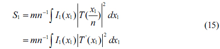
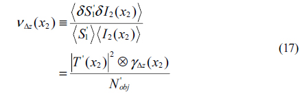
Based on the analysis above, we try to present a setup (Fig. 1(b)) which can eliminate the adverse effects of speckle size. In Fig. 1(b), the reference beam remains intact, and an optical modulator M is added to the object beam. The M is used to modulate the distribution of the light, and it can be a spatial light modulator (SLM) or lens, simply. Then the bucket signal can be rewritten as

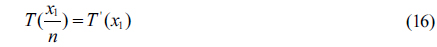
Where I₁'(x₁) = mI₁(nx₁) represents the modulated light field, m and n are the modulation coefficients. By converting the variable, we have the following result

The difference between Eq. (1) and Eq. (15) is the transmission function T '(x), which indicates that the modulation of the light is equivalent to the modulation of the object. When n > 1, the effect is to narrow the object. When n < 1, the effect is to amplify the object. So we have the following formula

This setup has at least three advantages: Firstly, we can arbitrarily zoom the object by setting different n. This feature allows us to image an object whose size is lager than the size of the detector. Secondly, according to Eq. (17), when n >, 1 / N'_obj > N_obj which illustrates that the improved setup has a higher visibility than the traditional setup. Thirdly, because the reference beam remains intact, the width of the edge blur remains δx₀ / 2.

Two independent experiments were implemented with the setups shown in Figs. 1(a) and (b), respectively. The two objects have the same size (slit, 1 mm × 3 mm). In Fig. 1(b), we used a concave lens as the modulator M and n = 2.12. The results are shown in Fig. 5. Panels a1 and b1 are results of the traditional ghost imaging while Panels a2 and b2 represent results of the improved method. The visibility of results in Panels a1 and b1 is about 0.0026, and the visibility of results in Panel a2 and b2 is about 0.012. We can see the improved ghost imaging has higher SNR and visibility (about 4.5 times) than the traditional ghost imaging by comparing the results. The improvement of visibility is due to the change of modulation coefficient n. Moreover, Panels b1 and b2 show that the two retrieved image have the same width of edge blur. However, there is a price to pay, which is the retrieved image is a narrowed object. The experimental results are in good agreement with the theoretical analysis results.

[FIG. 5.] The ghost imaging reconstruction of a 1 mm × 3 mm slit. (a1) and (b1) are the reconstruction image of the traditional setup, obtained with 16000 realizations. (a2) and (b2) are the reconstruction image of the improved setup, obtained with 16000 realizations.

III. CONCLUSION

In this paper, the impact of speckle size of pseudo-thermal light source on ghost imaging is theoretically and experimentally analyzed. For the same number of independent realizations, the larger speckle size of thermal source is, the higher visibility and SNR of the retrieved image and the more serious edge blur of the retrieved image will be. This means that the impact of the speckle size of the pseudothermal on GI is double-sided. In order to eliminate the adverse effects of the speckle size, we use a concave lens to modulate the object beam, which is equivalent to modulating the object. By the improved setup, we implement the experiment in which the experimental results are in good agreement with the theoretical analysis results.

참고문헌

1. Pittman T. B., Shih Y. H., Strekalov D. V., Sergienko A. V. (1995) “Optical imaging by means of two-photon quantum entanglement,” [Phys. Rev. A] Vol.52 P.3429-3432
2. Bennink R. S., Bentley S. J., Boyd R. W. (2002) “Two-photon coincidence imaging with a classical source,” [Phys. Rev. Lett.] Vol.89 P.113601
3. Gatti A., Brambilla E., Bache M., Lugiato L. A. (2002) “Ghost imaging with thermal light: comparing entanglement and classical correlation,” [Phys. Rev. Lett.] Vol.93 P.93602
4. Valencia A., Scarcelli G., D’Angelo M., Shih Y. (2005) “Two-photon imaging with thermal light,” [Phys. Rev. Lett.] Vol.94 P.063601
5. Ferri F., Magatti D., Gatti A., Bache M. (2005) “High-resolution ghost image and ghost diffraction experiments with thermal light,” [Phys. Rev. Lett.] Vol.94 P.183602
6. Basano L., Ottonello P. (2006) “Experiment in lensless ghost imaging with thermal light,” [Appl. Phys. Lett.] Vol.89 P.091109
7. Ferri F., Magatti D., Sala V. G., Gatti A. (2008) “Longitudinal coherence in thermal ghost imaging,” [Appl. Phys. Lett.] Vol.92 P.261109
8. Bromberg Y., Katz O., Silberberg Y. (2009) “Ghost imaging with a single detector,” [Phys. Rev. A] Vol.79 P.053840
9. Meyers R., Deacon K. S., Shih Y. (2008) “Ghost-imaging experiment by measuring reflected photons,” [Phys. Rev. A] Vol.77 P.041801(R)
10. Katz O., Bromberg Y., Silberberg Y. (2009) “Compressive ghost imaging,” [Appl. Phys. Lett.] Vol.95 P.131110
11. Zerom P., Wai K., Chan C., Howell J. C. (2011) “Entangledphoton compressive ghost imaging,” [Phys. Rev. A] Vol.84 P.061804(R)
12. Katkovnik V., Astola J. (2012) “Compressive sensing computational ghost imaging,” [J. Opt. Soc. Am. A] Vol.29 P.1556-1567
13. Cheng J. (2009) “Ghost imaging through turbulent atmosphere,” [Opt. Express] Vol.17 P.7916-7921
14. Bina M., Magatti D., Molteni M. (2013) “Backscattering differential ghost imaging in turbid media,” [Phys. Rev. Lett.] Vol.110 P.083901
15. Ferri F., Magatti D., Lugiato L. A. (2010) “Differential ghost imaging,” [Phys. Rev. Lett.] Vol.104 P.253603
16. Erkmen B. I., Shapiro J. H. (2009) “Signal-to-noise ratio of Gaussian-state ghost imaging,” [Phys. Rev. A] Vol.79 P.023833
17. Magatti D., Gatti A., Ferri F. (2009) “Three-dimensional coherence of light speckles: Experiment,” [Phys. Rev. A] Vol.79 P.053831
18. Gatti A., Magatti D., Ferri F. (2008) “Three-dimensional coherence of light speckles: Theory,” [Phys. Rev. A] Vol.78 P.063806

OAK XML 통계

이미지 / 테이블

[ FIG. 1. ] Experimental setups for ghost imaging. (a) the traditional setup for ghost imaging. (b) the improved setup for ghost imaging.
[ ]
[ ]
[ ]
[ ]
[ FIG. 2. ] The schematic view of the point x2 where the transmission function is T(x2) = 0.
[ ]
[ ]
[ ]
[ FIG. 3. ] The graph of │μ│2 vs │x1 ？ x2│.
[ ]
[ ]
[ ]
[ ]
[ ]
[ ]
[ FIG. 4. ] The ghost imaging reconstruction of an aperture whose diameter is 900 μm. (a1) and (b1) are the reconstruction images which obtain 12800 realizations, when the speckle size of the thermal source is 50 μm. (a2) and (b2) are the reconstruction image which obtain 12800 realizations, when the speckle size of the thermal source is 100 μm.
[ ]
[ ]
[ ]
[ ]
[ FIG. 5. ] The ghost imaging reconstruction of a 1 mm × 3 mm slit. (a1) and (b1) are the reconstruction image of the traditional setup, obtained with 16000 realizations. (a2) and (b2) are the reconstruction image of the improved setup, obtained with 16000 realizations.