Recent efforts to use the light-emitting diode (LED) in visible light communications (VLC) offer a new alternative for short-range communications that conveys information via light intensity [1, 2]. The original purpose of the lighting invokes an inherent constraint whereby the average optical intensity matches the dimming requirement imposed by a user. There have been a number of studies to achieve transmission techniques satisfying the constraint based on binary modulations [3-6], which are normally subject to limitations in the data rate. Therefore, the need for a higher data rate naturally leads to the use of multi-level modulations [7],1) such as pulse-amplitude modulation (PAM), and poses a new challenge for efficient multi-level modulation adapting to the dimming requirement.

One of the major challenging issues in LED research is efficiency droop [8]. In particular, nitride-based LEDs suffer from a reduction of internal quantum efficiency with increasing input, which results in saturation of output optical power. This phenomenon becomes one of the main obstacles to widespread deployment of gallium nitride (GaN)-based LEDs in lighting applications. Although this brings forth an impairment in terms of data rate for the communications feature, any impact on VLC has not been fully investigated. Droop causes impairment of energy efficiency and cooling, and failure in devices. Moreover, it negatively affects communications in two aspects: on nonlinear electrical-to-optical conversion and by reducing optical range. In theory, an LED’s output optical range determines communications capacity, whereas input signal, in practice, is processed in the electrical domain prior to nonlinear conversion. Both aspects are important, and an electrical signal should be carefully designed to maximize capacity with consideration of nonlinear conversion for the optical signal. This paper considers this detrimental effect on intensity-modulation-based optical communications and presents a design approach for an efficient modulation scheme equipped with an adaptation to the arbitrary dimming requirement. To this end, the maximally achievable rate of a VLC channel under efficiency droop is first presented, and optimization with the objective of maximizing the data rate is formulated. In view of the peak intensity restriction for VLC transceivers [7], this optimization naturally ends up as a simple convex problem that can be solved efficiently and exactly. This approach enables us to identify the optimal modulation for VLC channels.

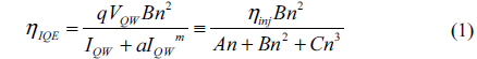
The numerical model of LED droop was first presented by Piprek [8] and is briefly introduced here. LED efficiency indicates a transfer ratio between the electrical and optical energies. However, the LEDs suffer from loss of electrons and photons during this transfer process. Accordingly, the total quantum efficiency, η _EQE is given by η _EQE = η _IQEη _EXE. Here, η _IQE is the internal quantum efficiency (IQE) and means the ratio of photons generated by electron-hole recombination to the total number of electrons injected into the LED which is related to electron loss. And η _EXE is the optical extraction efficiency (EXE) and means the ratio of photons emitted into free space to the total number of photons generated by the electron-hole recombination process. Efficiency droop is mainly caused by a gradual decrease in IQE as the injection current density surpasses typical values ranging between 0.1 and 10 A/cm² [9]. IQE can be further defined as the fraction of the total injected current to the current that feeds radiative recombination I_rad. The total current is split into carriers that recombine by generating photons, I_rad, and carriers that are lost to other non-radiative processes, such as Shockley-Read-Hall (SRH) recombination and Auger recombination inside quantum wells (QWs) and carrier leakage outside QWs. Accordingly, the total current injected into the LED is the sum of these four current components, which is the basis for the principal droop mechanism where I_rad is exceeded by others for increasing injection current. The sum of the first three current components inside QWs, denoted by I_QW, can be expressed with an ABC model [8] given by I_QW = qV_QW(An+Bn²+Cn³), where q is the electron charge, V_QW is the active volume of all QWs, and n is the carrier concentration. A, B, and C represent SRH recombination, radiative recombination, and the Auger coefficient, respectively. As for leakage current sources for a droop-causing mechanism, many have been supposed, including asymmetry in electron and hole transport, electron-attracting properties of the electron blocking layer, electron escape from the QW, and lack of electron capture into QWs [9]. Because the leakage current is not simply described in a simple equation, a simple relationship of the leakage current I_leak to I_QW is fitted [8] in the form I_leak = aI_QW^m. Therefore, the overall expression for IQE is given by

where injection efficiency η _inj is given by η _inj = I_QW / (I_QW + aI_QW^m), thereby accounting for the leakage. For the mathematical formulation, the electrical input and the optical output are denoted by U and X, respectively. We consider Eq. (1) as η _IQE = X(n) / U(n). Thus, Eq. (1) corresponds to a parametric form (or an implicit function) for the relationship between U and X. To obtain the relationship of an explicit function X ≡ g(U), which is independent of parameter n, we fix n to evaluate the numerator and denominator of Eq. (1) and to set as the output and input, respectively. This can be repeated for increasing n until a smooth curve is obtained. The results do not depend on n and are used to define explicit function X ≡ g(U).

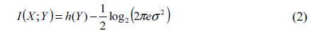
An efficient multi-level modulation is designed based on optimization with respect to symbol levels. Let X be the optically modulated signal communicated with VLC. From the practical consideration of intensity modulation [10], the signal levels of X are assumed to be upper- and lower-bounded, i.e., all symbols are contained in a non-negative finite range of signal levels. The optical signal undergoes a communications channel that can be modeled [11] with an additive white Gaussian noise (AWGN) channel. Then, the signal received at the photodetector (denoted by Y) is expressed as a corrupted version of X by additive noise Z with zero mean and standard deviation σ, i.e., Y=X+Z. The best achievable data rate for this AWGN channel is known to equal the mutual information [12] between channel input X and output Y, numerically evaluated using

where the first term is differential entropy h(Y) of channel output Y. Therefore, the design objective is to find the best set of symbol levels for X, such that the data rate in Eq. (2) is maximized under several constraints resulting from signal detection, dimming support, efficiency droop, etc. Note that channel output Y has a continuous probability distribution expressed as a mixture of multiple Gaussian distributions, and thus, the expression for data rate in Eq. (2) involves an integral. Therefore, determining the best configuration of X in an integral objective is very challenging. However, it is known that the best input distribution for an AWGN channel with bounded input levels has nonzero probabilities only at a finite set of input values [13, 14]. In other words, distribution of X has nonzero values only at a few separated levels. Therefore, the resulting multi-level modulation naturally resembles PAM, except that spacings between symbol levels are not uniform.

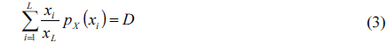
Multi-level modulation is assumed to have, at most, L different levels. However, the exact number of symbol levels (denoted by M) is unknown. Let x_i be the i-th smallest level of X. Thus, x₁ and x_L correspond to the zero level and the highest level that the optical transmitter emits, respectively. The dimming requirement whereby the mean intensity of the optical signal is equal to D∈[0, 1], set externally by a user, is expressed as

where p_X(x_i) is the probability that X takes the value of x_i. In addition, differential entropy h(Y) in Eq. (2) becomes

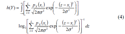
Let U be an electrical signal of a communications message. Because of efficiency droop in the optical intensity modulation using LED, electrical signal U undergoes distortion during the modulation. The resulting optical signal X is assumed to have a relationship with electrical signal U such that X=g(U). Therefore, the main goal readily reduces to the determination of the best distribution of U, such that the resulting electrical signal, or optical one, can convey the maximum amount of information via VLC. It is naturally speculated that the best distribution of U has uneven probabilities at discrete levels of a symbol, according to the preceding argument on X. Thus, U is assumed to take L different symbol levels based on the relationship x_i = g(u_i). In addition, the probability of U taking the i-th level u_i is denoted by p_i. Then, it holds that p_X(x_i) = p_X(g(u_i)) = p_i.

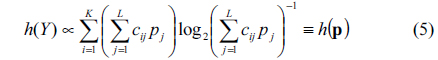
Next, for ease of numerical evaluation, the integral in Eq. (4) is discretized into a numerical integration. A finite interval of width 2σz_max, symmetric about the peak, is considered instead of [-∞, ∞]. Then, the finite interval is quantized with uniformly spaced K levels, and its two ends are defined as Δ₁ = x₁ - σz_max, and Δ_K = x_L + σz_max. The configuration of parameters z_max = 5, and K = L = 100 suffices to yield solutions of reasonable speed and accuracy, although K should be in fact chosen sufficiently larger than L. The discrete version of Eq. (4) is simply given by

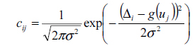
with coefficient c_ij given by

Note that function h(p) can be a new objective function, and can easily prove convex with respect to each pj. Therefore, the final optimization is given by

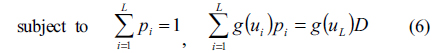
where two constraints result from the probability condition on U and the dimming constraint. Note that function xlogx and all affine (or linear) functions are convex and that their compositions, i.e., functions obtained by applying the output of one function as an input to the other function, and a linear combination of those compositions are also convex. Therefore, the objective function is concave [14]. Since all constraint functions are linear, i.e., convex, and the objective function is simply converted to a convex form by minimizing its negative, Eq. (6) corresponds to a convex optimization problem [15]. Therefore, any convex optimization solver package [16] can exactly obtain the optimal solution of Eq. (6). After the solution is found, the set of such levels that have nontrivial probability (p_i > 0) out of L levels is collected, and modulation order M is automatically determined by its cardinality. Normally, values of p_ij, j=1,…, M are not uniform, whereas communications messages are chosen uniformly. Therefore, pre-processing such as inverse source coding [6] is applied to convert messages so they have the obtained optimal distribution before optical modulation.

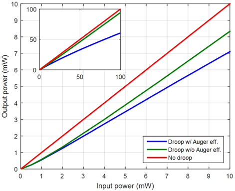
Numerical results are presented for various ranges of dimming target and data rate. First, the input-output relationships for three different droop models are depicted in Fig. 1. Model parameters are given as follows [8]: A=1ⅹ10⁷ , B=2ⅹ10^-11, C=1.5ⅹ10^-30, a=0.05 and m=1.58. The first model considers all effects caused by all parameters, while the second model does not consider the Auger effect, i.e., no cubic effect. The third model corresponds to the linear relationship between input and output. Here, the maximum output level is set at 10. The input-output relationship varies with respect to the range of input as the efficiency changes gradually. The slope in a lower-intensity regime is steeper than in a higher-intensity regime.

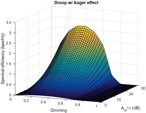
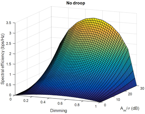
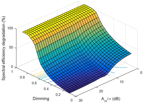
The maximum data rates for VLC transmission over a no-droop channel and a cubic-effect droop channel are illustrated with respect to dimming target d and A_m/σ in Figs. 2 and 3, where A_m is the maximum value of X. A_m/σ represents the channel or signal quality, where A_m is the signal range and σ is the noise standard deviation. The square of A_m/σ follows the dimension of the conventional signal-to-noise ratio. The CVX package [16] is used to solve Eq. (6). Note that the result is globally optimal because of the convexity of the optimization formulation. The resulting data rates are almost symmetric with respect to the range of dimming targets. Spectral efficiency keeps increasing, despite the efficiency droop, and reaches 2.7 bps/Hz at A_m/σ = 30 dB. Figure 4 depicts degradation in the data rate of VLC systems that is caused by droop. Since high dimming targets cannot be achieved in situations with efficiency droop, the loss in data rate is 100% for such dimming target regions. Furthermore, in dimming target regions that can be achieved even with efficiency droop, the data rate becomes very low, and the resulting loss is large, compared with situations without efficiency droop. It can also be observed that the loss is larger in a higher noise-power regime. This can be explained based on the shape of the probability distribution of signal Y, which determines differential entropy h(Y) in Eq. (2). If noise power is high, Y is dispersed in a wide region. Efficiency droop causes shrinkage of the spacing between consecutive data symbol levels. Thus, the tails of the resulting distribution of Y on the outside of the data signal region for X, i.e., [0, 10] for situations without droop in this example, remain nearly the same, whereas the probability distribution of Y within the data signal region for X changes significantly. Since the integral region of Y shrinks within the data signal region, i.e., [0, 7.2] for situations with droop in this example, the resulting differential entropy of Y decreases. In other words, the portion of Y that contributes to the integral evaluated in calculating the differential entropy is shortened by efficiency droop. The probability distribution of Y is merged within the data signal region by efficiency droop, and the resulting differential entropy decreases. In high-noise situations with Y dispersed widely, the distribution of Y has heavy tails, and the contribution of the probability distribution of the data signal region to the integral for the differential entropy is relatively high. Therefore, degradation of the differential entropy becomes high. By contrast, in low-noise situations where the distribution of Y is concentrated about data symbol levels, the values of probability distribution within the data signal region are mostly close to zero, and shrinkage of the integral region hardly changes the probability distribution of Y for this region. Thus, the change in the value of the integral is relatively small, and differential entropy is degraded little. Therefore, the loss of the data rate is larger in higher-noise situations.

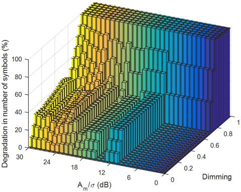
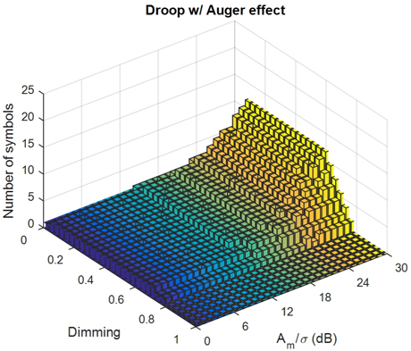
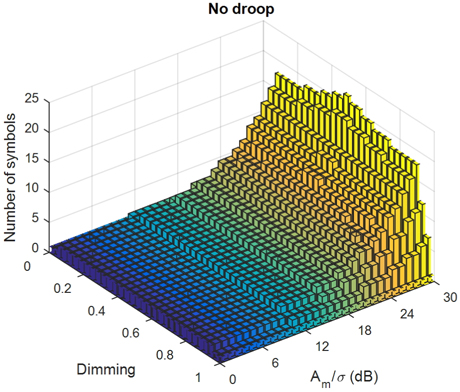
Figures 5 and 6 show the number of symbol levels for the optimal modulations of various dimming and noise configurations. We can see that the number of symbols for the optimal scheme is finite [13, 14], and the corresponding signal distribution is discrete. The number of symbols increases in low noise-power regimes. This can be understood as follows. In order to obtain maximal entropy h(Y) in Eq. (2), received signal Y should be spread as uniformly as possible. Since the communications channel is an additive noise, the tails in the distribution of received signal Y depend on the positions of symbols for transmitted signal X, and thus, received signal Y needs to be spread beyond the available region where the symbol of transmitted signal X can be placed. To this end, it is desirable for the two outmost symbols of transmitted signal X to be placed at two ends of the available region. In low-noise situations where received signal Y is not spread widely, many symbols for transmitted signal X need to be uniformly spread in the available signal region so the resulting distribution assimilates with the uniform distribution having the largest differential entropy. On the other hand, in high-noise situations where the distribution of received signal Y has long heavy tails, a small number of symbols for transmitted signal X is sufficient to ensure that the resulting distribution is spread widely. Thus, symbols of transmitted signal X are placed far from the center of the available symbol region. Therefore, high-noise situations lead to binary symbol mapping with two symbols placed at the two ends and, as noise power decreases, signal distributions with more symbols placed in between are created. This observation evidences the results of discrete distribution. As the noise power decreases, the number of modulation symbols increases. In most cases of low A_m/σ, binary on-off keying modulation is still a good transmission scheme for both droop and no-droop models. However, for a low-noise regime with good signal quality, almost all levels have nonzero probability values, i.e., the distribution becomes similar to uniform distribution. In addition, the number of symbols increases drastically for a good signal-quality regime, while other regions have only a few levels. This implies that analog-like modulation is very efficient for very good-quality regions, while the efficiency droop decreases the density of the information that can be conveyed with a given power. Figure 7 shows the decrease in symbol numbers according to efficiency droop. In a high dimming target region close to 1, the dimming target cannot be achieved, and the resulting number of symbols is zero. Therefore, degradation becomes 100%. In a region of low dimming targets and high noise power, the number of data symbols is two, regardless of the existence of efficiency droop, and degradation is 0%. In a low dimming target region, the number of data symbols increases from 2 to 3 and 4 as noise power decreases. Since the rate of the increase is higher in situations without efficiency droop, there are some regions where the resulting number of symbols is 3 without droop, but 2 with droop, thereby causing a 33% decrease in the number of symbols. Subsequently, if the number of symbols for droop situations becomes 3, the resulting degradation becomes 0%. Likewise, the degradation becomes 25% if the resulting number of symbols is 4 in situations without efficiency droop. Therefore, the overall degradation in the number of data symbols fluctuates, as shown in Fig. 7.

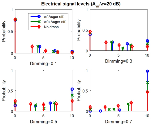
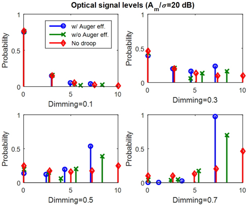
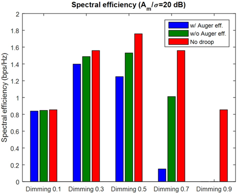
Figures 8 and 9 show the symbol-level distributions for electrical and optical signals, respectively, for several configurations of target dimming rate. The horizontal axis represents power values shown in Fig. 1. In conversion from an electrical signal to an optical signal, droop decreases the width of the signal span, i.e., the symbol region. Also, the symbol spacing between consecutive symbol levels of the optical signal becomes non-uniform. In addition, we can see that the number of symbols decreases in situations with efficiency droop. Figure 10 compares the data rates among different models for several target dimming values. We see that some regions of high dimming targets cannot be achieved with efficiency droop, and performance degradation is remarkable with high dimming targets.

This paper presents a multilevel transmission scheme for VLC systems implemented using an LED with efficiency droop. To find the best transmission scheme, convex optimization is formulated and solved using a simple convex solver package. Numerical results show that, although the droop incurs various impairments in devices, a substantial decrease in communications capacity can be minimized if the signal is carefully designed.