In the modern world, one is faced with innumerable problems arising from existing socioeconomic conditions that involve varying degrees of imprecision and uncertainty. We often need to take decisions in conflicting situations based on uncertain, ambiguous, or incomplete information. Human beings have a tremendous capability to form rational decisions based on such imprecise information. It is hard to formalize these human capabilities. This challenge has motivated us to consider a game theoretic model under conditions of uncertainty.

Game theory problems under uncertainty have been considered by many researchers, e.g., Nayak and Pal [1–3], Narayanan [4], and Nishizaki [5]. Narayanan [4] solved a 2 × 2 interval game using the probability and possibility approach but no certain distribution function has been used. Nayak and Pal [3] established a method of solution of a matrix game using interval numbers. But the solution has been considered under a certain condition which has been obviated by the authors in their work [6]. Biswas and Bose [7] constructed a quadratic programming model under fuzzily described system constraints on the basis of degree of satisfaction. Veeramani and Duraisamy [8] suggested a new approach for solving fuzzy linear programming problem using the concept of nearest symmetric triangular fuzzy number approximations with preserve expected interval. But this approach is not efficient when a primal basic feasible solution is not in hand. Ebrahimnejad and Nasseri [9] overcame this shortcoming using a new algorithm. Iskander [10] proposed a new approach for solving stochastic fuzzy linear programming problem using triangular fuzzy probabilities. Apart from this Kumar and Kar [11], Marbini and Tavana [12], Ebrahemnijad and Nasseri [13] have contributed substantially to the application of fuzzy mathematics in operations research. However, there are many shortcomings in the above-mentioned techniques for solving game problems in uncertain situations. These can be categorized as follows:

We consider the theory of fuzzy sets to address the uncertainty that occurs in industrial problems or machine learning. It is unlikely that we always have complete knowledge about the domain set. For example, when we try to address an object as ‘beautiful,’ we may not have complete knowledge about the parameters by which the beauty of an object can be explained, or the parameters, if assumed, may not match other people’s choices, i.e., they may not be unique. However, the reliability of the information must be taken into consideration, and this aspect is lacking in the fuzzy set description. We use soft set theory or rough set theory to describe uncertain situations. However, we may not know the complete set of parameters E in the case of a soft set, i.e., there is an issue regarding the reliability of the information concerned. In the rough set description, the lower or upper approximation or boundary region may not always be described, because knowledge or information about the equivalence relation R or domain U are only approximations or assumptions, and may not be known in advance. Additionally, it is not guaranteed that the desired optimal solution will be compatible with industrial applications. Different optimization techniques give rise to different optimal results, and we can only compare these results with those obtained by existing techniques. We cannot, however, ensure that a technique gives an actual optimal solution that will be universally accepted. The main reason behind this is that we cannot address the uncertainty properly, and thus use a number of assumptions.

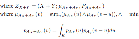
Thus, we need to develop the mathematical structures that provide a generalization of uncertain situations and that consider the reliability of available information. Zadeh [14] has made an attempt towards such a generalization by proposing Z-numbers. A Z-number is an ordered pair (A, B) in which A represents the restriction on a real-valued uncertain variable X and B is the measure of sureness, reliability, or certainty about A. However, the Z-number lacks informativeness when first introduced. Their composition in a summation has been defined [14], but the ranking or ordering of Z-numbers has not yet been considered. In this paper, we introduce a ranking of Z-numbers in the specific case where A represents a restriction on the measure of the possibility distribution with a Gaussian membership function, and B is a restriction on the probability measure with a normal density function. This ranking method is then used to solve a two-person zero-sum game using min − max and max − min principles [6] and the multi-section technique.

The remainder of this paper is organized as follows. In Section 2, we discuss the concept of Z-numbers, before presenting some basic definitions, notation, and comparisons related to interval numbers in Section 3. In Section 4, a matrix game with Z-numbers is proposed, and then Section 5 discusses the interval approximation of Z-numbers, and introduces some definitions, explanations, theorems about matrix games with Z-numbers, pure and mixed strategies, and saddle points. In section 6, a computational procedure is proposed along with a min-max algorithm, max-min algorithm, and multi-section technique. Section 7 presents an example in support of the proposed method, along with discussions related to our algorithm and the results of the numerical example. Brief conclusions are given in Section 8.

Let us consider a fuzzy set defined over a universe of discourse X. How will we define if X is not known in advance? Again, if it is assumed that X is known with certain parameters, then what is the reliability of such an information? We may say that we can define as type−2 fuzzy set where, X is a type−1 fuzzy set. In that case, X is also defined over some domain set . However, what will happen if is also not known? In Z-number representation, we may always construct X with some arbitrary element x ∈ X with some probability or possibility p. In that case, we can always associate a statement x with some statement G as

x is Gisλ

where, λ acts as a fuzzy quantifier and we consider it as probability induced by some possibility membership and we write

prob(x is G) = λ (fuzzy granularity [15]).

This situation, inspires us to define a Z-number formally. A Z-number Z is defined [14] as an ordered pair (A, B) where A and B are two fuzzy numbers and a Z-valuation is defined as

where, X is a real-valued uncertain variable, A is a restriction on the real values of the uncertain variable X and B is the reliability or certainty of A. Here, we consider X to be a random variable, A_X to be a restriction on the measure of a possibility distribution with membership function µ_AX and p_X is the restriction on probability distribution(density) function of X. The scalar product µ_AX .p_X gives the probability measure, P_AX of A_X and it is given as

Here, we recall that B is a restriction on the probability measure of A and it is not a restriction on the probability of A. Here, we attempt to ordering of the Z-numbers. For that purpose, here we consider the membership function as gaussian membership function. The reason behind taking such a function as membership function is that it is non-linear in nature and assume the situation which occurs generally in industrial applications. Unless otherwise stated by Z-number we here understand Z-valuation. For the sake of computation here we will consider a Z-number as (X ; A_X, P_AX ) or (X ; µ_AX , P_AX ) or(X ; <c, σ>, P_AX ) where c and σ are parameters of the Gaussian membership function. Here we may consider some examples like (Population of India, about 1200 million, very likely ),(degree of satisfaction, very high, not sure) which are considered as Z-number.

To consider an arithmetic operation, let Z_X = (X ; µ_AX , P_AX ) and Z_Y = (Y ; µ_AY , P_AY ) be two Z-numbers. Using the extension principle as described by [14], we obtain

Z_X + Z_Y = Z_X+Y

Let us consider that ℜ represents the set of all real numbers. We define an interval, Moore [16], as

where a_L and a_R are said to be the lower and upper limits of the interval , respectively. If a_L = a_R then is reduced to a real number a, where a = a_L = a_R . Corresponding interval arithmetic is given by 3.

For,

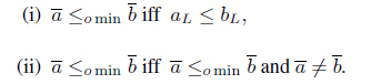
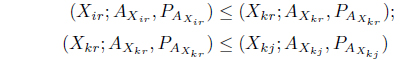
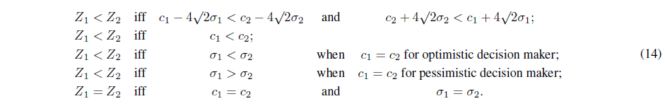
The order relation of interval numbers is discussed in several literature [16, 17]. Recently Chakrabortty et al. [18] proposed a revised definition of order relations between interval costs(or times) for minimization problems and interval profits for maximization problems for optimistic and pessimistic decision making. Let us suppose, the intervals and represent the uncertain interval costs (or times) or profits in center-radius form.

For minimization problems the order relation ‘ ≤_{o min}’ between the intervals and is

This implies that is superior to and is accepted. This order relation is not symmetric.

In pessimistic decision making, the decision maker expects the minimum cost/time for minimization problems according to the principle ‘Less uncertainty is better than more uncertainty’.

For minimization problems, the order relation ‘ <_{p min}’ between the intervals and is

(i) iff , for type-I and type-II intervals, (ii) iff and , for type-III intervals.

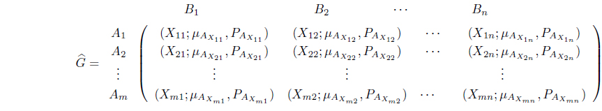
which is said to be matrix game with Z-numbers.

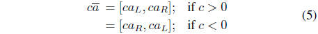
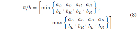
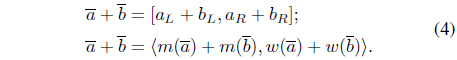
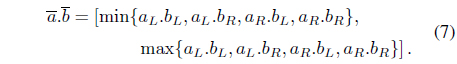
In this paper, arithmetic operations on interval [a, b] and their ranking as proposed in [6] serves as a level−1 computation [14] and the same is used in ranking of Z-numbers. Gregorzewski [19] proposed a method for interval approximation of fuzzy number. Here, in same way, we will approximate a Gaussian fuzzy number to an interval number. For that, let us consider a Gaussian fuzzy number <x, µ(x; c, σ)|x ∈ X> where the membership function is given as

Now, we define an α-cut set A_α as A_α = {x : µ(x; c, σ) ≥ α}. Then,

and let us consider that and . Let [a, b] be the corresponding interval approximation. Then

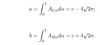
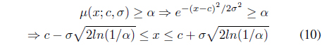
Therefore, if Z = (X; A_X, P_AX ) be a Z-number with Gaussian membership function µ(x; c, σ) then the corresponding interval approximation is and

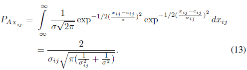
Here, we get the probability density function p_Xij as the normal density function N(c_ij , σ). Hence,

where . Then, we obtain from Eq. (9) that

Now, let us consider two Z-numbers Z₁, Z₂ and corresponding interval approximations as and Using the interval arithmetic, we propose the ranking of Z-numbers as

Suppose, the pay-off for player A in a matrix game with Z-number be represented as (X_ij ; A_Xij , P_AXij ). Then, the corresponding interval approximation will be given by . The pay-off matrix with elements as interval approximation of Z-number can then be represented as

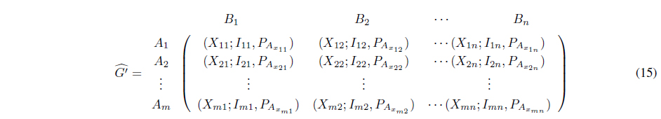
where , i = 1, 2 · · · m, j = 1, 2, · · · n and

Theorem 4.1. If Z₁(X₁; A_X1 , P_AX1 ) ≤ Z₂(X₂; A_X2 , P_AX2) then P_AX1 ≥ P_AX2 for optimistic decision maker and P_AX1 ≤ P_AX2 for pessimistic decision maker.

Proof. From the expression in (13) we see that P_AXij depend only on σ_ij and not on c_ij. Using this fact and combining the relation in (14) we can easily construct the proof of the theorem.

Notes: Here it should be noted that for pessimistic decision maker the degree of certainty P_AX is lesser iff the membership value or the interval approximation is lesser and for optimistic decision maker the degree of certainty does not matter at all, it only gives the degree of reliability of the information.

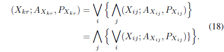
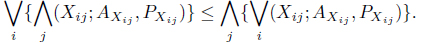
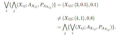
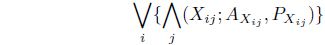
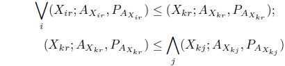
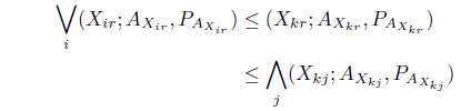
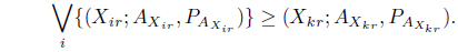
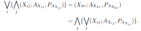
In the context of Z-number, a pure strategy may be considered as a decision making rule in which one particular course of action is selected with some degree of reliability or certainty for the pay off considered. Actually, Z-number gives higher level of generality compared to interval numbers where length of the interval actually measures the certainty. For lack of informativeness of Z-number, we develop the concept of pure strategy in the domain of interval numbers with parallel computation. For matrix game with Z-number, we define the min max and max min as

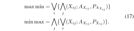
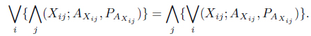
where ‘∨' and ‘∧' the max and min operators for two Z-number in the domain of Z-numbers Z respectively. In accordance with ranking of Z-numbers in (14), for games such as with pure strategy, we define the concept of saddle point solution.

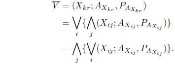
Definition 4.1. (Saddle Point) The concept of saddle point in classical form was proposed by Von Neumann and Morgenstern [20]. The (k, r)th position of the pay-off matrix with Z-numbers is said to be a saddle point of the matrix game , if and only if,

The position (k, r) is said to be a saddle point, the entry itself [a_kr, b_kr] represents the value of the game (denoted by ) and the pair of pure strategies leading to it are optimal pure strategies. Now we have to confirm that the relation as defined here for the saddle point solution actually exists for the matrix game with Z-numbers. For that purpose we must consider the following theorems.

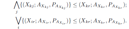
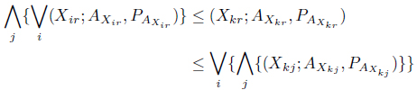
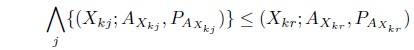
Theorem 4.2. Let ; i = 1, 2, ..., m; j = 1, 2, ..., n be the m × n pay-off matrix for a two-person matrix game Γ with Z-numbers. Suppose and both exist. Then

Proof. For some fixed i, we have, by using the order relation on Z,

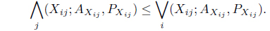
From (19) and (20) we have,

Here, we see that is independent of j, since (X_ij; A_Xij , P_Xij) has obtained minimum value for some fixed value of j. Hence we write

Again, the right-hand side of (21) is independent of i, hence, we obtain

Hence the theorem.

Theorem 4.3. Let both

and

exist. Then a necessary and sufficient condition that (X_ij; A_Xij , P_Xij) will be a saddle point at i = k, j = r is

and

Proof. Condition is necessary: Let

Let i = k make a maximum and let j = r make a minimum. Then, we write

As, , we have . Also, using the order relation over Z-numbers in Z,

This is one of the conditions for (X_ij; A_Xij , P_AXij) to have a saddle point. The other condition can similarly be deduced.

Condition is sufficient: Let (X_kr; A_Xkr , P_AXkr) be the saddle point of the pay-off matrix , then for i = k, j = r we have, by definition of saddle point

or,

or,

or,

as

and

Using the above Theorem 4.2 we have,

Hence the necessary and sufficient condition for the existence of a saddle point is proved.

Example 4.1. Let us consider the 2 × 2 matrix game with Z-number having the pay-off matrix as in the following:

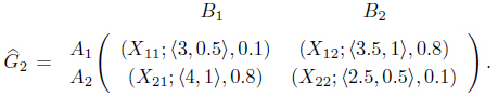
It can be easily verified that Therefore, the matrix game with Z-number has a saddle point at (1, 1) and the optimal strategies for players A and B are the pure strategies A₁ and B₁, respectively. The value of the matrix game is

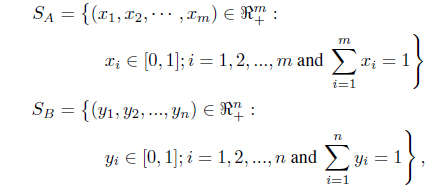
In a situation where the saddle point of a pay off matrix does not exist we allow mixed strategies to get a solution. In mixed strategies, the probability with which a player chooses a particular strategy is considered. In the context of Z-number, we can say that in mixed strategy game we find an expected pay off with some reliability or certainty of the pay off obtained. Suppose and be the m and n dimensional vector spaces, respectively. We denote x = (x₁, x₂, ··· , x_m)^T and y = (y₁, y₂, ..., y_n)^T , respectively, where the symbol ‘T' denotes the transpose of a vector. The strategy spaces for players A and B are denoted as

respectively. Vectors x ∈ S_A, y ∈ S_B are called mixed strategies of players A and B, respectively. Now, we should remember that Z-number is a higher(level 3) level of generality [14] and all the operational rules like multiplication, division are not known. In that case, it is better idea to find the mixed strategy solution using the interval approximation. Interval is a particular case of a Z-number and it is level−1 domain of computation. Now, the question may arise: Does an optimal mixed strategy solution with interval numbers actually correspond to an optimal mixed strategy solution with Z-numbers? To get an answer to this question we must consider the following theorem where, a Z-number is modelled with a gaussian membership function and normal probability density function.

Theorem 4.4. An optimal solution of the matrix game with pay-off elements as interval approximation of some Z-number corresponds to the optimal solution of the matrix game with pay-off elements the concerned Z-number.

Proof. Let us consider a maximization problem where, the elements of the pay off matrix are interval approximation of Z-numbers. Let us construct an interval approximation function ϕ : Z → I(ℜ). Now, the author’s [19] approach of interval approximation assures that the set of such functions is nonempty. We first establish that ϕ is a bijective mapping. Let Z₁, Z₂ ∈ Z. We can then find c₁, c₂, σ₁, σ₂ ∈ ℜ such that

Using interval arithmetic, we can easily verify that ϕ(Z₁) = ϕ(Z₂) ⇒ c₁ = c₂ and σ₁ = σ₂. Hence Z₁ = Z₂. Therefore, ϕ is injective.

Similarly, using interval arithmetic, we can easily verify that for every interval c₁, c₂, σ₁, σ₂ ∈ ℜ we can find Z₁, Z₂ ∈ Z, the set of solutions with Z-numbers, assuring that ϕ is surjective. Hence, ϕ is bijective. This property assures that every solution in I(ℜ) corresponds exactly to one solution in Z. Let I^∗ be the optimal solution of the maximization problem. Then, for every solution I, we must have,

Now, let us construct I and I^∗ as

Using equation (4.2) we have either

Since, ϕ is bijective we find Z^∗ such that Z ≤ Z^∗∀Z ∈ Z. Therefore, Z^∗ is the optimal solution of the maximization problem modelled by Z-numbers. Similar approach can be made for minimization problem. Hence the theorem is proved.

Note: We compute the inverse function , a Z-number ∀[a, b] ∈ ℜ which gives the optimal solution of the matrix game with Z-number corresponding to the optimal solution with interval number.

Definition 4.2. (Interval expected pay-off ): If the mixed strategies x = (x₁, x₂, ..., x_m) and y = (y₁, y₂, ..., y_n) are proposed by players A and B respectively, then the expected pay-off of the player A by player B is defined by

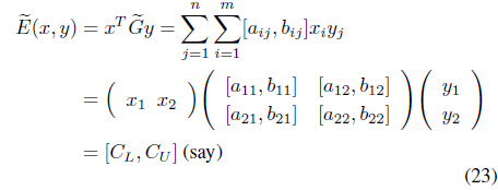
where,

CL = (a11 + a22 − b12 − b21)x1y1 + (a12 − b22)x1 + (a21 − b22)y1 + a22 CU = (b11 + b22 − a12 − a21)x1y1 + (b12 − a22)x1 + (b21 − a22)y1 + b22

The composition rules on interval numbers [6] are used in this definition (3) of expected pay-offs.

Definition 4.3. Suppose, and be two intervals defined over ℜ. Let us consider that there exist strategies x^∗ ∈ S_A, y^∗ ∈ S_B. If, for any strategy x ∈ S_A, y ∈ S_B, satisfies both

then, x ∈ S_A, y ∈ S_B, is said to be a reasonable solution to the interval matrix game and are called reasonable values for players A and B, respectively; x^∗ and y^∗ are called reasonable strategies for players A and B, respectively.

Let U and W be the sets of reasonable values for players A and B, respectively.

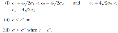
Definition 4.4. Let us consider that there exist two reasonable values and If there do not exist reasonable values and such that they satisfy both and , then is said to be a solution of the interval matrix game ; x^∗ is called an optimal (or a maximin) strategy for player A and y^∗ is called an optimal (or a minimax) strategy for player and are called Player A’s gain-floor and B’s loss-celling, respectively.

In this section, we discuss the computation procedure to find out the solution to a matrix game with Z-number. We first transform (through approximation) the pay off matrix with Z-numbers to a pay off matrix with corresponding interval-number. We then use multisection technique and min max algorithm [6] to solve the matrix game. The multisection algorithm is formulated according to the approach given in the work of Chakrabortty et al. [18]. The concept of multisection is inspired by the concept of multiple bi-section, where more than one bi-section is made at a single iteration cycle. The basis of this method is the comparison of intervals (as described in Section 3 of this paper) according to the decision makers point of view.

Algorithm for multisection technique

Input: λ(number of divisions), y, l(lower bound)and u(upper bound) of x.

Output: Probability x^∗

Step 1://calculation of step lengths//calculate step length h = (u − l)/λ

end for

Step 2://Division of concerned region into equal subregions //

Step 2.1: For j = 0 to λ − 1 Calculate l₀ = l + j ∗ h

Step 2.2: //Call the function C_L and C_U //.

Section 3,

Calculate C_L = lower value of the interval number ,

obtained by as in Eq.

(23)

Calculate C_U = upper value of the interval number ,

obtained by as in Eq.

(23)

Step 2.3: For j1 = 0 to λ − 1 Calculate l₁ = l + j1 ∗ h

Step 2.4: Calculate l_min = lower value of the interval number ,

obtained by as in Eq.

(23) at l₀

Calculate u_min upper value of the interval number ,

obtained by as in Eq.

(23) at l₀

Calculate C_l = lower value of the interval number ,

obtained by as in Eq.

(23) at l₁

Calculate C_u = upper value of the interval number ,

obtained by as in Eq.

(23) at l₁

Step 2.5: Applying required order relation (defined in Section 3)

between any two interval numbers [C_L, C_L] and [l_min, u_min] choose the optimal interval number.

end j1 loop

Step 2.6: Choose the subregion E^opt among E_j obtained in step 2.5 which has a better objective function value by comparing the interval values E_j to each other.

Step 3: //calculation of widths//.

Step 3.1: Calculate widths w_j = u_j − l_j of E_j where u_j and l_j are upper bounds and lower bounds of E_j

Step 3.2: While w_j > ε

break

Step 3.3: Set E^opt ← E_j

Return to step 2.1

end for

endwhile.

end j loop

Output

END MULTISECTION

On the basis of this technique we have developed an algorithm for max min and min max solutions of a single objective interval game.

Algorithm for min max principle

We conduct operations not on the degree of certainty P_{AXi j} but on interval numbers [6] using the following steps:

Step 1: Put y₁ = nh,where h = 1/M and n = 0, 1, 2, 3 ···

M = Number of divisions of the interval [0, 1]

Step 2: For n = i

Find max/optimistic order relation of ,

where 0 ≤ x₁ ≤ 1 by using multisection algorithm 4.1.

Step 3: Let the solution set for x is

Using pessimistic order relation find minimum of

Suppose it occurs at x₁ ^∗, which is a crisp number.

Step 4: Calculate

Step 5: Using pessimistic order relation calculate for 0 ≤ y₁ ≤ 1

by multisection technique. Suppose, the minimum value is (say).

Then (by Theorem 4.2) and

Therefore (x₁^∗, y₁^∗) is the optimal solution.

Algorithm for max min principle 4.2.1

Step 1: Put x₁ = nk, where k = 1/N and n = 0, 1, 2, 3, ···

N = number of divisions of the interval [0, 1]

Step 2: For n=i

Find min/pessimistic order relation of

where 0 ≤ y₁ ≤ 1 by using multisection technique 4.1.

Step 3: Let the solution set for y is

Using optimistic order relation find maximum of

Suppose it occurs at y₁ ^∗ , which is a crisp number.

Step 4: Calculate .

Step 5: Using optimistic order relation calculate

by multisection technique. Suppose the maximum value is (say).

Then (by Theorem 4.2) and

Therefore e (x₁^∗, y₁^∗) is the optimal solution.

Thus is a reasonable solution of the interval matrix game , is player A’s gain-floor and is player B’s loss-ceiling.

Suppose, a company conducts an opinion pole about an election. They place some questions in front of the voters and get answers as ‘We are not very sure that the candidate A’s honesty is high’ or ‘It is very likely that inflation during the period of the present government is high’. In such cases, we can consider the statements as (A’s degree of honesty, high, not sure) or (price hike, high, very likely). These conditions are representation of Z-numbers. When this happens between two candidates in an election, then it forms a matrix game with Z-number. Suppose, the pay-off matrix is given by

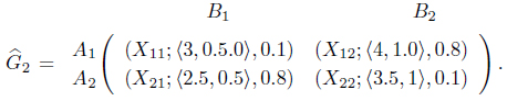
What are the optimal strategies and what is the value of game?

This is an example of 2 × 2 matrix game with Z-number which has no saddle point because

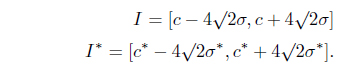
Using the definition of interval expected pay off (4.2) When we run min max and max min programmes in TURBOC we get the reasonable solutions as

x^∗ = (0.0.9375, 0.0625), y^∗ = (0.5, 0.5),

and

In this example, we obtain a reasonable solution

and

as respectively gain-floor and loss-ceiling of players A and B with the probabilities x^∗ = (0.0.9375, 0.0625), y^∗ = (0.5, 0.5). There is a significance behind the result obtained and the technique adopted.

(i) Here the pay off actually means some restriction on the measure of possibility that one can gain or loose with some degree of certainty and value of the game actually means measure of possibility of a solution to be an optimum solution. (ii) We have tried to arrive at a reasonable solution with some degree of certainty which is compatible with the real world situation as most of the optimization results obtained with other numbers or intervals lack some compatibility with the real world situation. For example, there are several kinds of imprecisions. What imprecision will then be modelled using a particular approach is a matter of concern as compared to the existing techniques [6]. In our approach, we have tried to consider a typical imprecision by using Z-number. (iii) We have tried to arrive at a higher degree of generality in the decision making process by using Z-number.

In a decision-making process, the information is often found to be imprecise, incomplete, e.g., ‘about 5%’, ‘high price” etc. In such a situation it is unlikely that usual approach would give a desired result. Again, formalization of the imprecision hardly occurs in our optimization models and there is no universal model which can consider all types of imprecisions. We often model certain types of imprecise data with certain type of membership function or interval numbers. It does not, however, ensure the optimization universally, i.e., there may be a chance to arrive at a better optimal solution if we model it otherwise. So, there is a need for formalization of imprecision and for that purpose we have used Z-number as a pay off which actually gives the degree of certainty. On the restriction of the measure of possibility of pay off one would gain or loose. Though we have modelled a Z-number with a particular type of membership and density function there is scope of further generalization. There is also scope for using this procedure to solve multi-objective decision-making problems.