The study of the emission patterns of gamma-ray pulsars has progressed ever since their discovery. There have been different models proposed in the past to explain the high energy radiation, i.e. the polar cap model (Ruderman & Sutherland 1975), the outer gap model (Cheng et al. 1986a, 1986b) and the slot gap model (Arons 1983). And, ever since the launch of the Fermi gamma-ray telescope, the study of gamma-ray pulsar emission patterns has become much easier. The large area telescope (LAT) on board Fermi has now detected gamma-ray photons from over 150 pulsars (Ackermann et al. 2015). The study of Romani & Watters (2010) showed that by comparing the computed pulse profiles with observations, it could be confidently stated that the outer gap model is more consistent than the slot cap model, although neither of these models can explain all the features of gamma-ray pulsars. Spectral fits of pulsars have showed that the observed spectrum is fitted well by a power law with a super-exponential cut-off (with a form of dN/dE∝E^−a exp[−(E/E_c)^b]). For different outer gap models, there is one common idea, that is, the electric field along the magnetic field is raised from charged-deficit regions. And, a portion of the curvature photons converted into electron/positron pairs that limited the size of the outer gap; thus, the size of the outer gap cannot take the entire open field line region (Cheng et al. 1986a, b; Zhang & Cheng 1997).

A previous model, the simple two-layer outer gap model (Wang et al. 2010), was used to study the phase-averaged spectrum of pulsars. In this model, the outer gap is considered as a combination of a main acceleration region and a screening region. The charge density distribution of the outer gap was assumed to be a simple step function. The acceleration region has a charge density much lower than the Goldreich-Julian density and is nearly a vacuum, which raises a strong electric field; particles are accelerated and curvature photons with energy in the GeV range are emitted. The particles produced by the pair creation process stop the growth of the acceleration region and form the screening region, which produce photons with energy of around 100 MeV. However, this can only explain the phase-averaged spectra, not the phase-resolved spectra. A previous study has considered the azimuthal structure of the outer gap (Wang et al. 2011) and the phase-resolved spectra and light curves of pulsars. In their work, they tested their model using the Vela pulsar, which has an energy dependent third peak in the light curve. The model successfully explained the phase-averaged spectra, the phase-resolved spectra, and the light curve.

One study has shown that non-thermal X-ray emission from the outer magnetosphere could be generated by Inverse-Compton Scattering between primary particles in the gap and the radio waves coming towards the pulsar (Ng et al. 2014). When the energy of the primary particles is large enough, the Inverse-Compton Scattering is capable of producing GeV photons.

In this paper, we assume, based on the three-dimensional two-layer outer gap model, that the magnetosphere of a pulsar is time-dependent. Instead of solving a time-dependent Poisson equation, we assume that one of the spectral parameters has a power-law distribution. For a certain value of the parameter we assign a possibility. Hence when we consider the distribution of the parameter, we can obtain a weighted spectrum. And, using the Inverse-Compton Scattering component, we can calculate the high energy tail of powerful pulsars.

This paper is organized as follows. In section 2, we present a simple non-stationary two-layer three-dimensional outer gap model. Here, instead of solving a time-dependent Poisson equation, we choose to give a probability distribution to the outer gap structure, showing that the structure of the outer gap changes over time. Then, to explain the slow dropping high energy tail of Geminga pulsar, we discuss the Inverse Compton Scattering component in relation to the high energy part. In section 3, we present the model fitting results of the non-stationary model and the model combining the Inverse-Compton Scattering component. In sections 4 and 5, we present the discussion and conclusions.

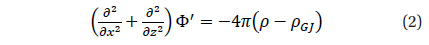
It is known that the outer gap extends from the last open field lines to the region between the null charge surface and the light cylinder. The previous study by Wang et al. (2010, 2011) assumed that the outer gap can be divided into two parts, the acceleration and the screening regions. They assumed that in the trans-field direction the charge density would have a simple step function, as shown below:

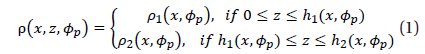
In the acceleration region, the charge density is assumed to be around 10% of the Goldreich-Julian density, thus producing a large electric field that accelerates the particles to ultra-relativistic velocity and produces GeV curvature photons. In the screening region, which is around the upper boundary, the charge density is larger than the Goldreich-Julian density due to the pair creation process.

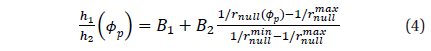
When we assume that the physical quantities change slowly in the azimuthal angle ϕ_p, this model becomes again a two dimensional one. Under the two dimensional model, using certain boundary conditions, the acceleration electric field can be obtained. Thus the curvature radiation spectrum can be derived from this electric field. In their work , Wang et al . (2010, 2011) derived three independent factors f, h₁/h₂, and 1−g₁ , which represent the fractional gap size, the ratio between the thicknesses of the acceleration region and the total gap size, and the number density in the acceleration region, respectively. With gradual change of the value of ϕ_p, the azimuthal structure of the outer gap can be solved for, and the azimuthal distribution of the three parameters can be written as:

Here we have five spectral parameters, C, B₁, B₂, (, and F. Combining these with the inclination angle and the viewing angle, one report (Wang et al. 2011) found that there are a total of seven parameters that we need to fix for the spectrum. They applied this model to the Vela pulsar and found that the model could successfully explain the phase-resolved spectrum and the energy-dependent third peak in the pulsar’s light curve.

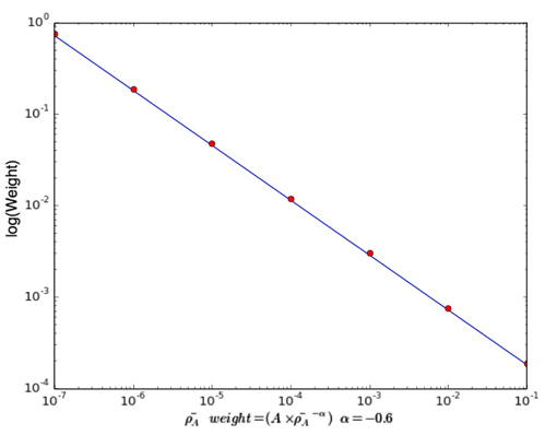
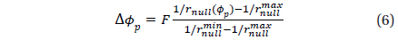
However, when we tried to apply this model to the Geminga pulsar, we found that when the energy of the photons exceeded the cutoff energy, the spectrum dropped faster than expected, which means that if this model is used, a flux of above GeV photons will be underestimated . We introduced the non-stationary model to solve this problem. We believe that the structure of the outer gap is not stationary, but changes from time to time. In this case, the Poisson equation needs to add a dimension for time, and by solving the time-dependent Poisson equation, this can be the model we are looking for. However, solving time-dependent Poisson equations is very complicated. In a simple case, we can assume a distribution for one of the spectral parameters proposed above. For one chosen parameter, we can assume a power-law distribution, P∝A∙x^−α, where x represents the parameter, A is a normalization factor, α is the power index decided by fitting the spectrum, and P is the weighting factor of a certain value of x. For each of the spectra with different x, we add the parameters together with the weighting factor and we can obtain the spectrum of the non-stationary model.

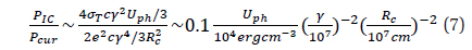
Although to some degree the non-stationary model can explain the spectral property of gamma ray pulsars, we noticed that for some very powerful pulsars like the Geminga pulsar there were difficulties. Ng et al. (2014) discovered that besides synchrotron radiation from secondary pairs in the outer gap, there is another way to produce X-ray emission for millisecond pulsars with large magnetic fields: Inverse-Compton Scattering between the radio emission and the primary particles in the outer gap. According to their study, as the radio, X-ray, and gamma ray emission regions are likely to be at the same positions, so the radio waves emitted from the outer gap can, then, scatter with the primary particles with ultra-relativistic energy. To compare this energy with the curvature radiation from the outer gap, we may argue as follows.

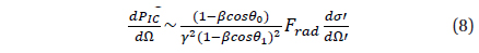
We can conclude from this equation that the flux predicted by Inverse-Compton Scattering has about the same magnitude as the curvature radiation, and thus is observable for the pulsars. To calculate the Inverse-Compton Scattering spectrum, Ng et al. (2014) considered the scattering between the outwards primary particles and the outwards radio waves. The radio emission region is assumed to be just above the outer gap; for each particle, the power per unit energy per unit solid angle of the Inverse-Compton scattering is

Here dσ'/dΩ' is the Klein-Nishina cross section, is the collision angle between the particles and the radio photons, 0<θ₁<1/γ is the angle between the direction of the particle motion and the direction of the scattered photons, and F_rad is the radio spectrum.

As we can see from Eq. (8), the spectrum of Inverse-Compton Scattering relies a lot on the radio spectrum. Although this spectrum is currently unknown, it is suggested that at a low frequency of less than 1 GHz, there will be a turnover point in the spectrum at around 100 MHz for millisecond pulsars (Kuzmin & Losovsky 2001); we set this frequency as the turnover value. After comparing the theoretical results with the observations, we here assume a broken power-law radio spectrum:

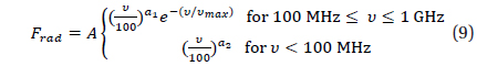
We also set the spectral indexes a₁=−2.7 and a₂=0.5 according to observations. A is a normalization factor we select; it can vary by a factor of a few , because the exact pattern of the radio emission is unknown.

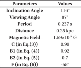
In this section, we apply our model to the Geminga pulsar. We chose to give a power-law distribution to the charge density, in Eq. (5). In the previous study we found that the Geminga pulsar is very powerful, which means that it needs a large outer gap to provide its emission, and thus the fitted value of the fractional gap size (f) is very large. So, we decided not to change the gap size in this model and only assigned the power-law distribution to the charge density . We first decided on a set of parameters that fitted the best of the observed phase-averaged spectrum; we then changed . The other parameters are shown in Table 1. By fitting the weighted phase-averaged spectrum, we chose the power index α=0.8. The relation between and the weight factors is shown in Fig. 1. The weighted phase-averaged spectrum is shown in Fig. 2.

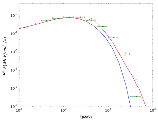
In Fig. 3, the combined spectrum of Inverse-Compton Scattering and the outer gap is presented. When combining the Inverse-Compton scattering spectrum with the curvature radiation, we add only the part above 1 GeV.

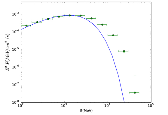
In the beginning we believed that the high energy emission of the Geminga pulsar would be explained by the non-stationary model; however, from the results it is obvious that this is far from the reality. Different distribution patterns of selected parameters may lead to even better results; however, if we still want to undertake a detailed study of this problem, we cannot avoid solving a time-dependent Poisson equation.

It is argued that most photons emitted from the gap are from above the null charge surface, as shown in the results above; however, fellow researchers have predicted that the inner boundary of the gap can extend inwards (Takata et al. 2004), which may also be the reason for the lack of high energy (above 3 GeV) photons.

In this paper, we discussed the non-stationary three dimensional two-layer outer gap model and used it to explain the high energy emission (above approximately 3 GeV) of the Geminga pulsar, observed by Fermi-LAT. The outer gap consists of a main acceleration region and a screening region, as studied by Wang et al. (2011); we have five spectral parameters. However, we extended the model, making it non-stationary. We assigned a power-law distribution to one of the spectral parameters and, for the Geminga pulsar, we decided that this parameter would be the charge density. We found that this method did not create a sufficient number of high energy photons, so we added an Inverse-Compton Scattering component to the model. This process can produce sufficient high energy photons, as has been shown above.